Chapter 5 Manuscript Preparation with RMarkdown in R
5.1 Publishing with R Markdown
Yihui Xie, who has written several of the most essential packages in this space, including knitr, first introduced R Markdown in 2012. Xie presents R Markdown as “an authoring framework for data science” in his book R Markdown: The Definitive Guide. The .Rmd file is used to automatically “save and execute code, as well as generate high-quality reports.” Documents and presentations in HTML, PDF, Word, Markdown, Powerpoint, LaTeX, and more formats are all supported. Homework assignments, journal articles, full-length books, formal reports, presentations, web pages, and interactive dashboards are just a few of the possibilities he offers, with examples of each. It is an understatement to suggest that it is a flexible and dynamic environment.
5.2 R Markdown Syntax
R Markdown files consist of the following elements:
- A metadata header that uses the YAML syntax to configure multiple output choices.
- Markdown-formatted content in the body
- Three
backticksseparate code chunks, which are separated by a curly braced block that identifies the language and sets chunk settings.
R Markdown also allows users to embed code expressions in the prose by enclosing them in single backticks. A minimal .Rmd example is included below. This is based on the Xie’s sample, which I’ve modified to demonstrate all of the elements mentioned above.
---
02: title: "Hello Dinsho"
03: author: "Mesfin Diro"
04: output: html_document
05: ---
06:
07: This is a paragraph in an _R Markdown_ document.
08: Below is a code chunk:
09:
10: ```{r fit-plot, echo=TRUE}
11: fit = lm(dist ~ speed, data = cars)
12: b   = coef(fit)
13: plot(cars)
14: abline(fit)
15: ```
16:
17: The slope of the regression is `r round(b[2], digits = 3)`.
R Markdown provides an authoring framework for data science. You can use a single R Markdown file to both
- save and execute code
- generate high quality reports that can be shared with an audience
R Markdown documents are fully reproducible and support dozens of static and dynamic output formats. This is an R Markdown file, a plain text file that has the extension
.Rmd.
 - The file contains three types of content:
1. An (optional) YAML header surrounded by
- The file contains three types of content:
1. An (optional) YAML header surrounded by ---s
2. R code chunks surrounded by ```s
3. text mixed with simple text formatting
5.3 Rendering output
- To generate a report from the file, run the render command:
library(rmarkdown)
render("example_1.Rmd)- Better still, use the “Knit” button in the RStudio IDE to render the file and preview the output with a single click or keyboard shortcut.r
R Markdown with Knit button in RStudio
- R Markdown generates a new file that contains selected text, code, and results from the .Rmd file. The new file can be a finished web page, PDF, MS Word document, slide show, notebook, handout, book, dashboard, package vignette or other format.
5.4 How it works

R Markdown with Knit button in RStudio
When you run render, R Markdown sends the
.Rmdfile to knitr, which runs all of the code chunks and generates a new markdown(.md)document with the code and its output.Knitr generates a markdown file, which is then processed by pandoc, which generates the final format.
While this may appear hard, R Markdown simplifies the process by combining all of the above processing into a single render function.
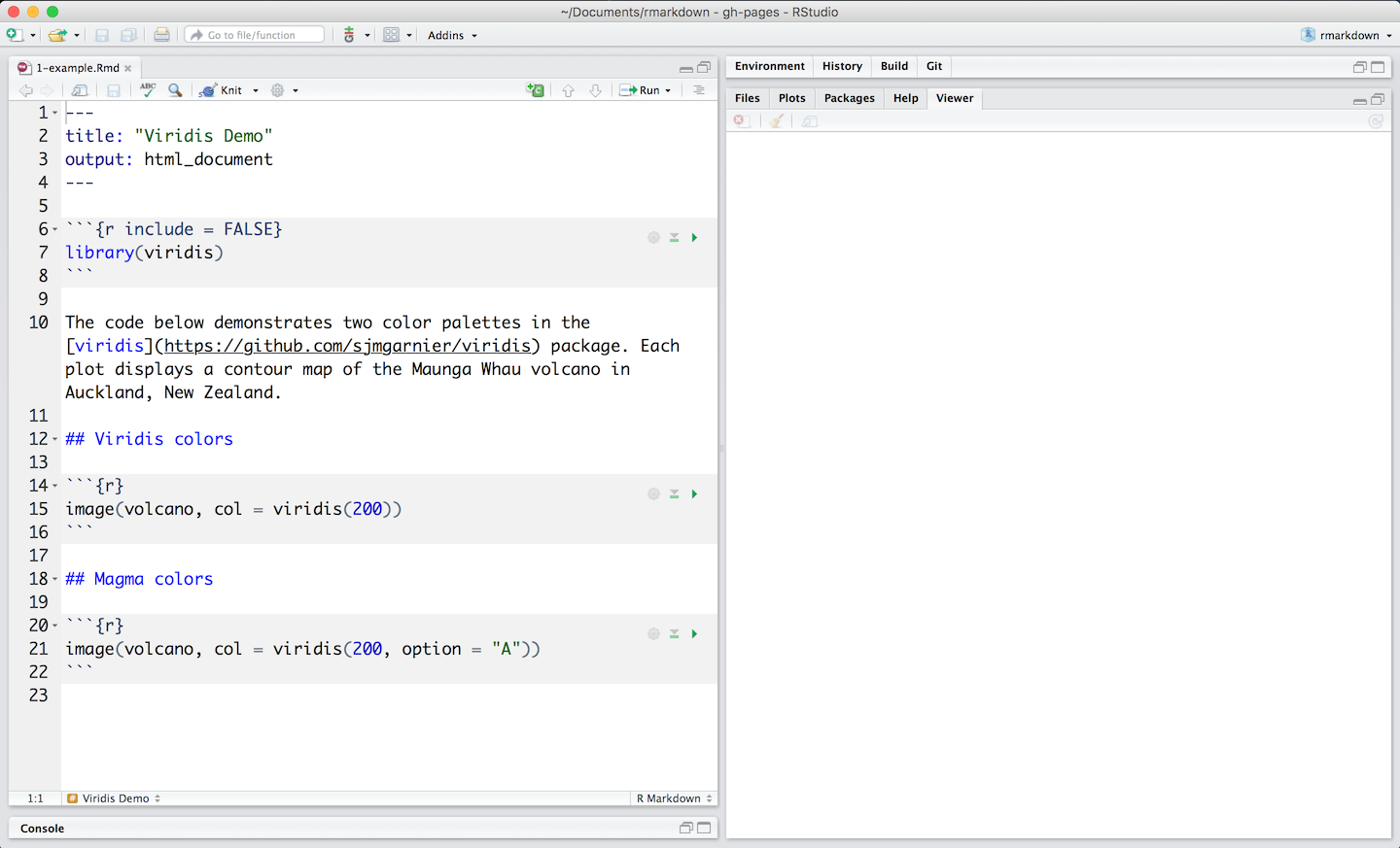
5.5 Code Chunks
- The R Markdown file below contains three code chunks:
R Markdown with Knit button in RStudio
- You can quickly insert chunks like these into your file with
- the keyboard shortcut Ctrl + Alt + I (OS X: Cmd + Option + I)
- the Add Chunk
 command in the editor toolbar or or by typing the chunk delimiters
 {r}__ and __.
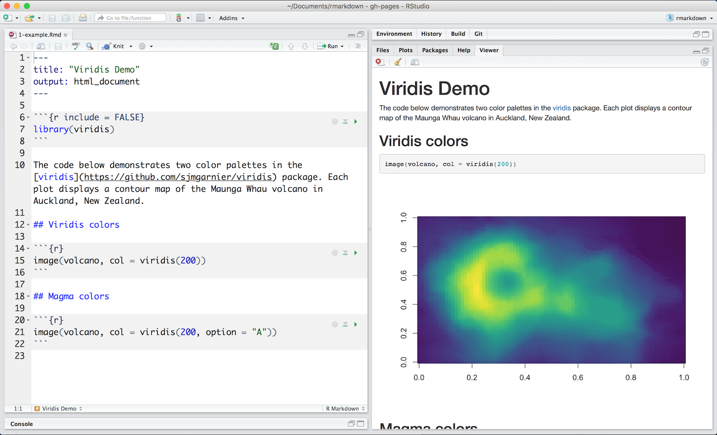
- When you render your .Rmd file, R Markdown will run each code chunk and embed the results beneath the code chunk in your final report.
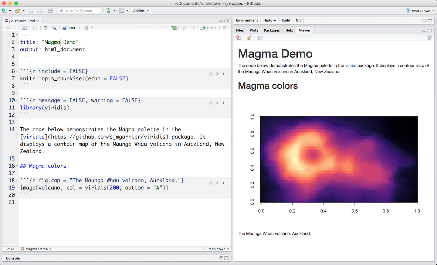
5.6 Inline Code
- Code results can be inserted directly into the text of a
.Rmdfile by enclosing the code with`r`. The file below uses`r`twice to call colorFunc, which returns “heat.colors”.

- Using
`r`makes it easy to update the report to refer to another function.
5.7 Code Languages
knitr can execute code in many languages besides R. Some of the available language engines include:
- Python
- SQL
- Bash
- Rcpp
- Stan
- JavaScript
- CSS
To process a code chunk using an alternate language engine, replace the
rat the start of your chunk declaration with the name of the language:
{bash}
5.8 Academic Journals
Academic publications frequently have severe formatting requirements for submitted articles. Few journals support R Markdown submissions directly at the moment, however several do support the LaTeX format. While you can convert R Markdown to LaTeX, different journals have different typesetting requirements and LaTeX styles, so it may be time-consuming and frustrating for all authors who want to use R Markdown to figure out the technical details of how to properly convert a R Markdown-based paper to a LaTeX document that meets the journal requirements.
The rticles package is designed to simplify the creation of documents that conform to submission standards. A suite of custom R Markdown templates for popular journals is provided by the package
5.8.1 Get started
You can install and use rticles from CRAN as follows:
# Install from CRAN
install.packages("rticles")

# Or install development version from GitHub
devtools::install_github("rstudio/rticles")
The development version of the package from GitHub is recommended because it has the most recent versions as well as various new templates.
If you’re using RStudio, go to File -> New File -> R Markdown to access the templates. This will bring up a dialog window where you may choose from a number of different templates.
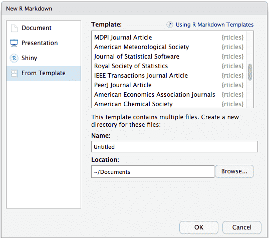
The R Markdown template window in RStudio showing available rticles templates
If you are using the command line, you can use the rmarkdown::draft() function, which requires you to specify a template using the journal short name, e.g.,
rmarkdown::draft(
  "JSSArticle.Rmd", template = "jss", package = "rticles"
)
5.8.2 rticles templates
The rticles package provides templates for various journals and publishers, including:
- R Journal articles
- CTeX documents
- JSS articles (Journal of Statistical Software)
- ACM articles (Association of Computing Machinery)
- ACS articles (American Chemical Society)
- AMS articles (American Meteorological Society)
- PeerJ articles
- Elsevier journal submissions
- AEA journal submissions (American Economic Association)
- IEEE Transaction journal submissions
- Statistics in Medicine journal submissions
- Royal Society Open Science journal submissions
- MDPI journal submissions
- Springer journal submissions
The full list is available within the R Markdown templates window in RStudio, or through the function rticles::journals():
library(rticles)
rticles::journals()
## [1] "acm" "acs" "aea" "agu"
## [5] "ajs" "amq" "ams" "arxiv"
## [9] "asa" "bioinformatics" "biometrics" "copernicus"
## [13] "ctex" "elsevier" "frontiers" "glossa"
## [17] "ieee" "ims" "informs" "iop"
## [21] "isba" "jasa" "jedm" "joss"
## [25] "jss" "lipics" "lncs" "mdpi"
## [29] "mnras" "oup_v0" "oup_v1" "peerj"
## [33] "pihph" "plos" "pnas" "rjournal"
## [37] "rsos" "rss" "sage" "sim"
## [41] "springer" "tf" "trb" "wellcomeor"