Chapter 3 Data Analysis with R
3.1 What is R? What is RStudio?
The term R is used to refer to both the programming language and the software that interprets the scripts written using it.
RStudio is a popular tool for not just writing R scripts but also interacting with the R software. RStudio requires R to function properly, thus both must be installed on your machine.
3.2 Why learn R?
3.2.1 R does not involve lots of pointing and clicking, and that’s a good thing
The learning curve may be longer than with other tools, but the outcomes of your research with R are based on a sequence of written commands rather than a series of pointing and clicking, which is a positive thing! So, if you want to redo your analysis because you gathered more data, you don’t need to remember which buttons you clicked in which order to get your results; all you have to do is rerun your script.
Working using scripts clarifies the steps you took in your investigation, and the code you write can be reviewed by another person who can provide input and point out errors.
Working with scripts challenges you to think more deeply about what you’re doing and makes it easier to learn and comprehend the approaches you utilize.
3.2.2 R code is great for reproducibility
When someone else (including your future self) can get the same results from the same dataset using the same analysis, it’s called reproducibility.
To generate manuscripts from your code, R interfaces with different technologies. The figures and statistical tests in your publication are automatically updated if you acquire more data or correct a mistake in your dataset.
Knowing R will offer you an advantage with these requirements, as an increasing number of journals and funding agencies seek repeatable analyses.
3.2.3 R is interdisciplinary and extensible
R provides a framework that allows you to integrate statistical methodologies from various scientific disciplines to best suit the analytical framework you need to examine your data, with over 10,000+ packages that can be installed to increase its capabilities. R, for example, contains packages for image analysis, geographic information systems (GIS), time series, population genetics, and much more.
3.2.4 R works on data of all shapes and sizes
The abilities you learn with R scale quickly as your dataset grows in size. It won’t make a difference to you if your dataset comprises hundreds or millions of lines.
R was created with data analysis in mind. It includes specific data structures and data types that simplify the handling of missing data and statistical elements.
R can connect to spreadsheets, databases, and a variety of other data formats, both locally and remotely.
3.2.5 R produces high-quality graphics
R’s plotting capabilities are limitless, allowing you to tweak every part of your graph to best convey the message from your data.
3.2.6 R has a large and welcoming community
R is used by thousands of people every day. Many of them are prepared to help you through mailing lists and websites such as Stack Overflow, or on the RStudio community.
3.2.7 Not only is R free, but it is also open-source and cross-platform
Anyone can look at the source code to learn more about R. Because of this transparency, there are less chances for errors, and you (or someone else) can report and repair faults if you find them.
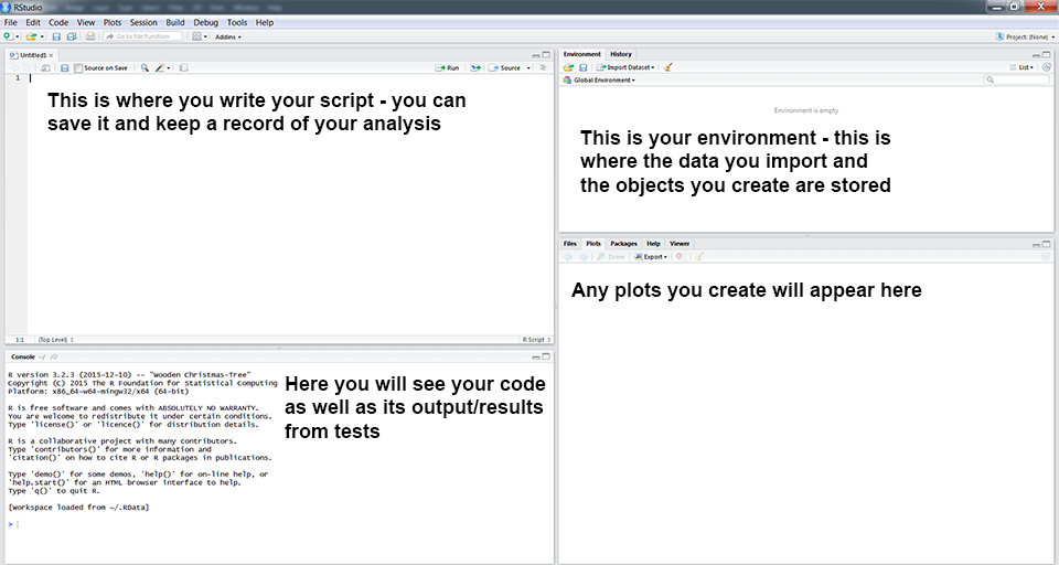
Rstudio Panels
3.2.8 Knowing your way around RStudio
Let’s begin by learning about RStudio, an Integrated Development Environment (IDE) for R programming.
The Affero General Public License (AGPL) v3 covers the RStudio IDE open-source project. A commercial license and priority email assistance from RStudio, Inc. are also available for the RStudio IDE.
We’ll use the RStudio IDE to write code, navigate our computer’s files, analyze the variables we’ll create, and visualize the plots we’ll make. Other features of RStudio that we will not cover during the course include version management, package development, and writing Shiny apps.
3.3 Introduction to R
You can get output from R simply by typing math in the console:
5 + 6## [1] 11 10 /3## [1] 3.333333However, we must give values to objects in order to accomplish useful and interesting things. To make an object, we must first give it a name, then use the assignment operator. <-, and the value we want to give it:
weight_kg <- 65<- is the assignment operator. It assigns values on the right to objects on the left. So, after executing x <- 3, the value of x is 3. The arrow can be read as 3 goes into x. For historical reasons, you can also use = for assignments, but not in every context. Because of the slight differences in syntax, it is good practice to always use <- for assignments.
In RStudio, typing Alt + - (push Alt at the same time as the - key) will write <- in a single keystroke in a PC, while typing Option + - (push Option at the same time as the - key) does the same in a Mac.
When assigning a value to an object, R does not print anything. You can force R to print the value by using parentheses or by typing the object name:
weight_kg <- 65    # doesn't print anything
(weight_kg <- 65)  # but putting parenthesis around the call prints the value of `weight_kg`
## [1] 65weight_kg # and so does typing the name of the object## [1] 65Now that R has weight_kg in memory, we can do arithmetic with it. For instance, we may want to convert this weight into pounds (weight in pounds is 2.2 times the weight in kg):
weight_lb <- weight_kg * 2.23.3.2 Functions and their arguments
Functions are “canned scripts” that automate more complex sets of commands, such as operations assignments and the like. Many functions are predefined or can be accessed by installing R packages (more on that later). A function typically takes one or more arguments as input. Most (but not all) functions return a value. The function sqrt() is an excellent example. The input (argument) must be an integer, and the output (return value) is the square root of that number. Calling a function (‘running it’) is the process of executing it. A function call might look like this:
ten <- sqrt(weight_kg)The sqrt() method is given the value of weight kg, which calculates the square root and returns the value, which is then assigned to the object ten. Because it just accepts one argument, this function is incredibly basic.
Let’s try a function that can take multiple arguments: round()
round(3.14159)## [1] 3We used round() with only one argument, 3.14159, and it returned 3. Because the default is to round to the nearest full number, this is the case. We can see how to gain extra digits by gathering knowledge about the round function. To find out what arguments it requires, we can use args(round) or search up the documentation for this method with ?round.
args(round)## function (x, digits = 0)
## NULLWe see that if we want a different number of digits, we can type digits = 3 or however many we want.
round(3.14159, digits = 3)## [1] 3.142# or
round(3.14159, 3)## [1] 3.1423.3.3 Data Structure
R has several core data structures, and we’ll take a look at each. * Vectors * Factors * Lists * Matrices/arrays * Data frames
3.3.3.1 Vectors
Vectors form the basis of R data structures. It is the most frequent and fundamental data type in R, and it is the workhorse of the language. A vector is made up of a collection of values that can be numbers or characters. The c() function can be used to assign a set of values to a vector. For instance, we may make a vector of animal weights and assign it to a new object called weight_g:
weight_g <- c(70, 80, 75, 22)
weight_g
## [1] 70 80 75 22A vector can also contain characters:
animals <- c("rat","mouse",  "dog")
animals
## [1] "rat" "mouse" "dog"The quotation marks surrounding “mouse,” “rat,” and other words are crucial. Without the quotations, R will presume that objects named rat, mouse, and dog have been created. There will be an error message since these objects do not exist in R’s memory.
There are numerous functions for inspecting the content of a vector. length() returns the number of elements in a given vector:
length(weight_g)## [1] 4length(animals)## [1] 3An important feature of a vector, is that all of the elements are the same type of data. The function class() indicates the class (the type of element) of an object:
class(animals)## [1] "character"class(weight_g)## [1] "numeric"The function str() provides an overview of the structure of an object and its elements. It is a useful function when working with large and complex objects:
str(weight_g)## num [1:4] 70 80 75 22str(animals)## chr [1:3] "rat" "mouse" "dog"You can use the c() function to add other elements to your vector:
weight_g <- c(weight_g, 10) # add to the end of the vector
weight_g <- c(20, weight_g) # add to the beginning of the vector
weight_g
## [1] 20 70 80 75 22 10Elements of an atomic vector are the same type. Example types include:
- character
- numeric (double)
- integer
- logical
3.3.4 Subsetting vectors
We must specify one or more indices in square brackets if we want to extract one or more values from a vector. Consider the following:
animals <- c("mouse", "rat", "dog", "cat")
animals[2]
## [1] "rat"animals <- c("mouse", "rat", "dog", "cat")
animals[c(3,1)]## [1] "dog" "mouse"We can also repeat the indices to create an object with more elements than the original one:
animals <- c("mouse", "rat", "dog", "cat")
animals[c(3,1, 2, 1, 3, 1,4)]
## [1] "dog" "mouse" "rat" "mouse" "dog" "mouse" "cat"R indices start at 1. Programming languages like Fortran, MATLAB, Julia, and R start counting at 1, because that’s what human beings typically do. Languages in the C family (including C++, Java, Perl, and Python) count from 0 because that’s simpler for computers to do.
3.3.5 Conditional subsetting
Another common way of subsetting is by using a logical vector. TRUE will select the element with the same index, while FALSE will not:
weight_g <- c(20, 10, 39, 54, 65)
weight_g[c(TRUE, FALSE, FALSE, TRUE, TRUE)]
## [1] 20 54 65weight_g > 40## [1] FALSE FALSE FALSE TRUE TRUEweight_g[weight_g > 40]## [1] 54 65You can combine multiple tests using & (both conditions are true, AND) or | (at least one of the conditions is true, OR):
weight_g[weight_g < 20 | weight_g > 60]## [1] 10 65weight_g[weight_g < 20 & weight_g == 60]## numeric(0)3.3.6 Missing Data
As R was designed to analyze datasets, it includes the concept of missing data (which is uncommon in other programming languages). Missing data are represented in vectors as NA.
When doing operations on numbers, most functions will return NA if the data you are working with include missing values. This feature makes it harder to overlook the cases where you are dealing with missing data. You can add the argument na.rm = TRUE to calculate the result while ignoring the missing values.
heights <- c(2, 4, 4, NA, 6)
mean(heights)
## [1] NAheights <- c(2, 4, 4, NA, 6)
mean(heights)## [1] NAmin(heights)## [1] NAmax(heights, na.rm = TRUE)## [1] 6If your data include missing values, you may want to become familiar with the functions is.na(), na.omit(), and complete.cases(). See below for examples.
# Extract those elements which are not missing values.
heights[!is.na(heights)]
## [1] 2 4 4 6# Returns the object with incomplete cases removed. The returned object is an atomic vector of type `"numeric"` (or `"double"`).
na.omit(heights)## [1] 2 4 4 6
## attr(,"na.action")
## [1] 4
## attr(,"class")
## [1] "omit"# Extract those elements which are complete cases. The returned object is an atomic vector of type `"numeric"` (or `"double"`).
heights[complete.cases(heights)]## [1] 2 4 4 63.3.6.1 Factors
An important type of vector is a factor. Factors are used to represent categorical data structures. Although not exactly precise, one can think of factors as integers with labels. For example, the underlying representation of a variable for sex is 1:2 with labels “Male” and “Female”. They are a special class with attributes, or metadata, that contains the information about the levels.
x = factor(c("Male","Female","Female","Male","Male"))
x
## [1] Male Female Female Male Male
## Levels: Female Maleattributes(x)## $levels
## [1] "Female" "Male"
##
## $class
## [1] "factor"The underlying representation is numeric, but it is important to remember that factors are categorical. Thus, they can’t be used as numbers would be, as the following demonstrates.
x_num = as.numeric(x)  # convert to a numeric object
sum(x_num)
## [1] 8Error in Summary.factor(c(1L, 1L, 1L, 1L, 1L, 1L, 1L, 1L, 1L, 1L, 2L, :
‘sum’ not meaningful for factors
Error in base::try(heights, silent = TRUE) : object 'heights' not found3.3.6.2 Logicals
Logical scalar/vectors are those that take on one of two values: TRUE or FALSE. They are especially useful in flagging whether to run certain parts of code, and indexing certain parts of data structures (e.g. taking rows that correspond to TRUE). We’ll talk about the latter usage later.
Here is a logical vector.
my_logic= c(TRUE, FALSE, TRUE, FALSE, TRUE, TRUE)
my_logic
## [1] TRUE FALSE TRUE FALSE TRUE TRUENote also that logicals are also treated as binary 0:1, and so, for example, taking the mean will provide the proportion of TRUE values.
!my_logic## [1] FALSE TRUE FALSE TRUE FALSE FALSEas.numeric(my_logic)## [1] 1 0 1 0 1 1mean(my_logic)## [1] 0.66666673.3.6.3 Numeric and Integer
The most common type of data structure you’ll deal with are integer and numeric vectors.
ints <- -3:3   # integer sequences are easily constructed with the colon operator
class(ints)
## [1] "integer"set.seed(42) # fix the random numbers seed
x <- rnorm(5) # 5 random values from the standard normal distribution
x## [1] 1.3709584 -0.5646982 0.3631284 0.6328626 0.4042683typeof(x)## [1] "double"class(x)## [1] "numeric"The main difference between the two is that integers regard whole numbers only and are otherwise smaller in size in memory, but practically speaking you typically won’t distinguish them for most of your data science needs.
3.3.6.4 Dates
The common data structure you’ll deal with is a date variable. Typically dates require special treatment and to work as intended, but they can be stored as character strings or factors if desired. The following shows some of the base R functionality for this.
Sys.Date()## [1] "2022-11-21"x = as.Date(c(Sys.Date(), '2022-05-25', Sys.Date()+2))
x## [1] "2022-11-21" "2022-05-25" "2022-11-23"In almost every case however, a package like lubridate will make processing them much easier. The following shows how to strip out certain aspects of a date using it.
library(lubridate)
month(Sys.Date())
## [1] 11library(lubridate)
day(Sys.Date())## [1] 21library(lubridate)
wday(Sys.Date()) # week start day ( 1-Monday, 7-sunday)## [1] 2quarter(Sys.Date())## [1] 4as_date('2022-01-01') + 100## [1] "2022-04-11"In general though, dates are treated as numeric variables, with consistent (but arbitrary) starting point. If you use these in analysis, you’ll probably want to make zero a useful value (e.g. the starting date)
as.numeric(Sys.Date())## [1] 193173.3.7 Matrices
With multiple dimensions, we are dealing with arrays. Matrices are two dimensional (2-d) arrays, and extremely commonly used for scientific computing. The vectors making up a matrix must all be of the same type. For example, all values in a matrix might be numeric, or all character strings.
3.3.7.1 Creating a matrix
Creating a matrix can be done in a variety of ways.
# create vectors
x <- 1:4
y <-  5:8
z <-  9:12

rbind(x, y, z)   # row bind
## [,1] [,2] [,3] [,4]
## x 1 2 3 4
## y 5 6 7 8
## z 9 10 11 12cbind(x, y, z) # row bind## x y z
## [1,] 1 5 9
## [2,] 2 6 10
## [3,] 3 7 11
## [4,] 4 8 12matrix(
c(x, y, z),
nrow = 3,
ncol = 4,
byrow = TRUE
)## [,1] [,2] [,3] [,4]
## [1,] 1 2 3 4
## [2,] 5 6 7 8
## [3,] 9 10 11 12matrix(
c(x, y, z),
nrow = 3,
ncol = 4,
byrow = FALSE
)## [,1] [,2] [,3] [,4]
## [1,] 1 4 7 10
## [2,] 2 5 8 11
## [3,] 3 6 9 123.3.8 Data Frames
Data frames are a very commonly used data structure, and are essentially a representation of data in a table format with rows and columns. Elements of a data frame can be different types, and this is because the data.frame class is actually just a list. As such, everything about lists applies to them. But they can also be indexed by row or column as well, just like matrices. There are other very common types of object classes associated with packages that are both a data.frame and some other type of structure (e.g. tibbles in the tidyverse).
Usually your data frame will come directly from import or manipulation of other R objects (e.g. matrices). However, you should know how to create one from scratch.
3.3.8.1 Creating a data frame
The following will create a data frame with two columns, a and b.
a <- c(1, 5, 2)
b <- c(3, 8, 1)
df <- data.frame(a,b)
df
## a b
## 1 1 3
## 2 5 8
## 3 2 1Much to the disdain of the tidyverse, we can add row names also
rownames(df) <- paste0('row',1:3)
df
## a b
## row1 1 3
## row2 5 8
## row3 2 1Everything about lists applies to data.frames, so we can add, select, and remove elements of a data frame just like lists. However we’ll visit this more in depth later, and see that we’ll have much more flexibility with data frames than we would lists for common data analysis and visualization.
3.4 Starting with data
We can read and load the data table from csv format:
library(tidyverse)
df <- read_csv("data/combined.csv")
This statement doesn’t produce any output because, as you might recall, assignments don’t display anything. If we want to check that our data has been loaded, we can see the contents of the data frame by typing its name: df
Wow… that was a lot of output. At least it means the data loaded properly. Let’s check the top (the first 6 lines) of this data frame using the function head():
head(df)## # A tibble: 6 × 13
## record_id month day year plot_id speci…¹ sex hindf…² weight genus species
## <dbl> <dbl> <dbl> <dbl> <dbl> <chr> <chr> <dbl> <dbl> <chr> <chr>
## 1 1 7 16 1977 2 NL M 32 NA Neot… albigu…
## 2 72 8 19 1977 2 NL M 31 NA Neot… albigu…
## 3 224 9 13 1977 2 NL <NA> NA NA Neot… albigu…
## 4 266 10 16 1977 2 NL <NA> NA NA Neot… albigu…
## 5 349 11 12 1977 2 NL <NA> NA NA Neot… albigu…
## 6 363 11 12 1977 2 NL <NA> NA NA Neot… albigu…
## # … with 2 more variables: taxa <chr>, plot_type <chr>, and abbreviated
## # variable names ¹species_id, ²hindfoot_lengthstr(df)## spc_tbl_ [34,786 × 13] (S3: spec_tbl_df/tbl_df/tbl/data.frame)
## $ record_id : num [1:34786] 1 72 224 266 349 363 435 506 588 661 ...
## $ month : num [1:34786] 7 8 9 10 11 11 12 1 2 3 ...
## $ day : num [1:34786] 16 19 13 16 12 12 10 8 18 11 ...
## $ year : num [1:34786] 1977 1977 1977 1977 1977 ...
## $ plot_id : num [1:34786] 2 2 2 2 2 2 2 2 2 2 ...
## $ species_id : chr [1:34786] "NL" "NL" "NL" "NL" ...
## $ sex : chr [1:34786] "M" "M" NA NA ...
## $ hindfoot_length: num [1:34786] 32 31 NA NA NA NA NA NA NA NA ...
## $ weight : num [1:34786] NA NA NA NA NA NA NA NA 218 NA ...
## $ genus : chr [1:34786] "Neotoma" "Neotoma" "Neotoma" "Neotoma" ...
## $ species : chr [1:34786] "albigula" "albigula" "albigula" "albigula" ...
## $ taxa : chr [1:34786] "Rodent" "Rodent" "Rodent" "Rodent" ...
## $ plot_type : chr [1:34786] "Control" "Control" "Control" "Control" ...
## - attr(*, "spec")=
## .. cols(
## .. record_id = col_double(),
## .. month = col_double(),
## .. day = col_double(),
## .. year = col_double(),
## .. plot_id = col_double(),
## .. species_id = col_character(),
## .. sex = col_character(),
## .. hindfoot_length = col_double(),
## .. weight = col_double(),
## .. genus = col_character(),
## .. species = col_character(),
## .. taxa = col_character(),
## .. plot_type = col_character()
## .. )
## - attr(*, "problems")=<externalptr>3.4.1 Inspecting Data Frame Objects
We already saw how the functions head() and str() can be useful to check the content and the structure of a data frame. Here is a non-exhaustive list of functions to get a sense of the content/structure of the data. Let’s try them out!
- Size:
dim(df)- returns a vector with the number of rows in the first element, and the number of columns as the second element (the dimensions of the object)nrow(df)- returns the number of rowsncol(df)- returns the number of columns
- Content:
head(df)- shows the first 6 rowstail(df)- shows the last 6 rows
- Names:
names(df)- returns the column names (synonym of colnames() for data.frame objects)rownames(df)- returns the row names Summary:str(df)- structure of the object and information about the class, length and content of each columnsummary(df)- summary statistics for each column
Note: most of these functions are “generic”, they can be used on other types of objects besides data.frame.
3.5 Indexing and subsetting data frames
Our survey data frame has rows and columns (it has 2 dimensions), if we want to extract some specific data from it, we need to specify the “coordinates” we want from it. Row numbers come first, followed by column numbers. However, note that different ways of specifying these coordinates lead to results with different classes.
# first element in the first column of the data frame (as a vector)
df[1, 1]
## # A tibble: 1 × 1
## record_id
## <dbl>
## 1 1# first element in the 6th column (as a vector)
df[1, 6] ## # A tibble: 1 × 1
## species_id
## <chr>
## 1 NL# first column of the data frame (as a vector)
df[, 1] ## # A tibble: 34,786 × 1
## record_id
## <dbl>
## 1 1
## 2 72
## 3 224
## 4 266
## 5 349
## 6 363
## 7 435
## 8 506
## 9 588
## 10 661
## # … with 34,776 more rows# first column of the data frame (as a data.frame)
df[1] ## # A tibble: 34,786 × 1
## record_id
## <dbl>
## 1 1
## 2 72
## 3 224
## 4 266
## 5 349
## 6 363
## 7 435
## 8 506
## 9 588
## 10 661
## # … with 34,776 more rows# first three elements in the 7th column (as a vector)
df[1:3, 7] ## # A tibble: 3 × 1
## sex
## <chr>
## 1 M
## 2 M
## 3 <NA># the 3rd row of the data frame (as a data.frame)
df[3, ] ## # A tibble: 1 × 13
## record_id month day year plot_id speci…¹ sex hindf…² weight genus species
## <dbl> <dbl> <dbl> <dbl> <dbl> <chr> <chr> <dbl> <dbl> <chr> <chr>
## 1 224 9 13 1977 2 NL <NA> NA NA Neot… albigu…
## # … with 2 more variables: taxa <chr>, plot_type <chr>, and abbreviated
## # variable names ¹species_id, ²hindfoot_length# equivalent to head_df <- head(df)
head_df <- df[1:6, ] : is a special function that creates numeric vectors of integers in increasing
or decreasing order, test 1:10 and 10:1 for instance.
You can also exclude certain indices of a data frame using the “-” sign:
df[, -1] # The whole data frame, except the first column## # A tibble: 34,786 × 12
## month day year plot_id species_id sex hindf…¹ weight genus species taxa
## <dbl> <dbl> <dbl> <dbl> <chr> <chr> <dbl> <dbl> <chr> <chr> <chr>
## 1 7 16 1977 2 NL M 32 NA Neot… albigu… Rode…
## 2 8 19 1977 2 NL M 31 NA Neot… albigu… Rode…
## 3 9 13 1977 2 NL <NA> NA NA Neot… albigu… Rode…
## 4 10 16 1977 2 NL <NA> NA NA Neot… albigu… Rode…
## 5 11 12 1977 2 NL <NA> NA NA Neot… albigu… Rode…
## 6 11 12 1977 2 NL <NA> NA NA Neot… albigu… Rode…
## 7 12 10 1977 2 NL <NA> NA NA Neot… albigu… Rode…
## 8 1 8 1978 2 NL <NA> NA NA Neot… albigu… Rode…
## 9 2 18 1978 2 NL M NA 218 Neot… albigu… Rode…
## 10 3 11 1978 2 NL <NA> NA NA Neot… albigu… Rode…
## # … with 34,776 more rows, 1 more variable: plot_type <chr>, and abbreviated
## # variable name ¹hindfoot_lengthdf[-c(7:34786), ] # Equivalent to head(df)## # A tibble: 6 × 13
## record_id month day year plot_id speci…¹ sex hindf…² weight genus species
## <dbl> <dbl> <dbl> <dbl> <dbl> <chr> <chr> <dbl> <dbl> <chr> <chr>
## 1 1 7 16 1977 2 NL M 32 NA Neot… albigu…
## 2 72 8 19 1977 2 NL M 31 NA Neot… albigu…
## 3 224 9 13 1977 2 NL <NA> NA NA Neot… albigu…
## 4 266 10 16 1977 2 NL <NA> NA NA Neot… albigu…
## 5 349 11 12 1977 2 NL <NA> NA NA Neot… albigu…
## 6 363 11 12 1977 2 NL <NA> NA NA Neot… albigu…
## # … with 2 more variables: taxa <chr>, plot_type <chr>, and abbreviated
## # variable names ¹species_id, ²hindfoot_lengthData frames can be subset by calling indices (as shown previously), but also by calling their column names directly:
df["species_id"]       # Result is a data.frame
df[, "species_id"]     # Result is a vector
df[["species_id"]]     # Result is a vector
df$species_id          # Result is a vector
In RStudio, you can use the autocompletion feature to get the full and correct names of the columns.
3.6 Factors
When we did str(df) we saw that several of the columns consist of
integers. The columns genus, species, sex, plot_type, … however, are
of a special class called factor. Factors are very useful and actually
contribute to making R particularly well suited to working with data. So we are
going to spend a little time introducing them.
Factors represent categorical data. They are stored as integers associated with labels and they can be ordered or unordered. While factors look (and often behave) like character vectors, they are actually treated as integer vectors by R. So you need to be very careful when treating them as strings.
Once created, factors can only contain a pre-defined set of values, known as levels. By default, R always sorts levels in alphabetical order. For instance, if you have a factor with 2 levels:
sex <- factor(c("male", "female", "female", "male"))R will assign 1 to the level "female" and 2 to the level "male" (because
f comes before m, even though the first element in this vector is
"male"). You can see this by using the function levels() and you can find the
number of levels using nlevels():
levels(sex)## [1] "female" "male"nlevels(sex)## [1] 2Sometimes, the order of the factors does not matter, other times you might want
to specify the order because it is meaningful (e.g., “low”, “medium”, “high”),
it improves your visualization, or it is required by a particular type of
analysis. Here, one way to reorder our levels in the sex vector would be:
sex # current order## [1] male female female male
## Levels: female malesex <- factor(sex, levels = c("male", "female"))
sex # after re-ordering## [1] male female female male
## Levels: male femaleIn R’s memory, these factors are represented by integers (1, 2, 3), but are more
informative than integers because factors are self describing: "female",
"male" is more descriptive than 1, 2. Which one is “male”? You wouldn’t
be able to tell just from the integer data. Factors, on the other hand, have
this information built in. It is particularly helpful when there are many levels
(like the species names in our example dataset).
3.6.1 Converting factors
If you need to convert a factor to a character vector, you use
as.character(x).
as.character(sex)## [1] "male" "female" "female" "male"In some cases, you may have to convert factors where the levels appear as
numbers (such as concentration levels or years) to a numeric vector. For
instance, in one part of your analysis the years might need to be encoded as
factors (e.g., comparing average weights across years) but in another part of
your analysis they may need to be stored as numeric values (e.g., doing math
operations on the years). This conversion from factor to numeric is a little
trickier. The as.numeric() function returns the index values of the factor,
not its levels, so it will result in an entirely new (and unwanted in this case)
set of numbers. One method to avoid this is to convert factors to characters,
and then to numbers.
Another method is to use the levels() function. Compare:
year_fct <- factor(c(1990, 1983, 1977, 1998, 1990))
as.numeric(year_fct)               # Wrong! And there is no warning...
## [1] 3 2 1 4 3as.numeric(as.character(year_fct)) # Works...## [1] 1990 1983 1977 1998 1990as.numeric(levels(year_fct))[year_fct] # The recommended way.## [1] 1990 1983 1977 1998 1990Notice that in the levels() approach, three important steps occur:
- We obtain all the factor levels using
levels(year_fct) - We convert these levels to numeric values using
as.numeric(levels(year_fct)) - We then access these numeric values using the underlying integers of the
vector
year_fctinside the square brackets
3.6.2 Renaming factors
In addition to males and females, there are about 1700 individuals for which the sex information hasn’t been recorded. Additionally, for these individuals, there is no label to indicate that the information is missing or undetermined. Let’s rename this label to something more meaningful. Before doing that, we’re going to pull out the data on sex and work with that data, so we’re not modifying the working copy of the data frame:
sex <- df$sex
head(sex)
## [1] "M" "M" NA NA NA NAlevels(sex)## NULLlevels(sex)[1] <- "undetermined"
levels(sex)## [1] "undetermined"head(sex)## [1] "M" "M" NA NA NA NA3.6.3 Using stringsAsFactors=FALSE
By default, when building or importing a data frame, the columns that contain
characters (i.e. text) are coerced (= converted) into factors. Depending on what you want to do with the data, you may want to keep these
columns as character. To do so, read.csv() and read.table() have an
argument called stringsAsFactors which can be set to FALSE.
In most cases, it is preferable to set stringsAsFactors = FALSE when importing
data and to convert as a factor only the columns that require this data
type.
## Compare the difference between our data read as `factor` vs `character`.
df <- read.csv("data/combined.csv", stringsAsFactors = TRUE)
str(df)
df <- read.csv("data/combined.csv", stringsAsFactors = FALSE)
str(df)
## Convert the column "plot_type" into a factor
df$plot_type <- factor(df$plot_type)
3.7 Formatting Dates
One of the most common issues that new (and experienced!) R users have is
converting date and time information into a variable that is appropriate and
usable during analyses. As a reminder from earlier in this lesson, the best
practice for dealing with date data is to ensure that each component of your
date is stored as a separate variable. Using str(), We can confirm that our
data frame has a separate column for day, month, and year, and that each contains
integer values.
str(df)We are going to use the ymd() function from the package lubridate (which belongs to the tidyverse; learn more here). . lubridate gets installed as part as the tidyverse installation. When you load the tidyverse (library(tidyverse)), the core packages (the packages used in most data analyses) get loaded. lubridate however does not belong to the core tidyverse, so you have to load it explicitly with library(lubridate)
Start by loading the required package:
library(lubridate)ymd() takes a vector representing year, month, and day, and converts it to a
Date vector. Date is a class of data recognized by R as being a date and can
be manipulated as such. The argument that the function requires is flexible,
but, as a best practice, is a character vector formatted as “YYYY-MM-DD”.
Let’s create a date object and inspect the structure:
my_date <- ymd("2015-01-01")
str(my_date)
## Date[1:1], format: "2015-01-01"Now let’s paste the year, month, and day separately - we get the same result:
# sep indicates the character to use to separate each component
my_date <- ymd(paste("2015", "1", "1", sep = "-"))
str(my_date)
## Date[1:1], format: "2015-01-01"Now we apply this function to the surveys dataset. Create a character vector from the year, month, and day columns of
df using paste():
date <- paste(df$year, df$month, df$day, sep = "-")
head(date)
## [1] "1977-7-16" "1977-8-19" "1977-9-13" "1977-10-16" "1977-11-12"
## [6] "1977-11-12"This character vector can be used as the argument for ymd():
date2 <- ymd(paste(df$year, df$month, df$day, sep = "-"))The resulting Date vector can be added to df as a new column called date:
df$date <- ymd(paste(df$year, df$month, df$day, sep = "-"))
str(df) # notice the new column, with 'date' as the class
## spc_tbl_ [34,786 × 14] (S3: spec_tbl_df/tbl_df/tbl/data.frame)
## $ record_id : num [1:34786] 1 72 224 266 349 363 435 506 588 661 ...
## $ month : num [1:34786] 7 8 9 10 11 11 12 1 2 3 ...
## $ day : num [1:34786] 16 19 13 16 12 12 10 8 18 11 ...
## $ year : num [1:34786] 1977 1977 1977 1977 1977 ...
## $ plot_id : num [1:34786] 2 2 2 2 2 2 2 2 2 2 ...
## $ species_id : chr [1:34786] "NL" "NL" "NL" "NL" ...
## $ sex : chr [1:34786] "M" "M" NA NA ...
## $ hindfoot_length: num [1:34786] 32 31 NA NA NA NA NA NA NA NA ...
## $ weight : num [1:34786] NA NA NA NA NA NA NA NA 218 NA ...
## $ genus : chr [1:34786] "Neotoma" "Neotoma" "Neotoma" "Neotoma" ...
## $ species : chr [1:34786] "albigula" "albigula" "albigula" "albigula" ...
## $ taxa : chr [1:34786] "Rodent" "Rodent" "Rodent" "Rodent" ...
## $ plot_type : chr [1:34786] "Control" "Control" "Control" "Control" ...
## $ date : Date[1:34786], format: "1977-07-16" "1977-08-19" ...
## - attr(*, "spec")=
## .. cols(
## .. record_id = col_double(),
## .. month = col_double(),
## .. day = col_double(),
## .. year = col_double(),
## .. plot_id = col_double(),
## .. species_id = col_character(),
## .. sex = col_character(),
## .. hindfoot_length = col_double(),
## .. weight = col_double(),
## .. genus = col_character(),
## .. species = col_character(),
## .. taxa = col_character(),
## .. plot_type = col_character()
## .. )
## - attr(*, "problems")=<externalptr>Let’s make sure everything worked correctly. One way to inspect the new column is to use summary():
summary(df$date)## Min. 1st Qu. Median Mean 3rd Qu. Max.
## "1977-07-16" "1984-03-12" "1990-07-22" "1990-12-15" "1997-07-29" "2002-12-31"
## NA's
## "129"Something went wrong: some dates have missing values. Let’s investigate where they are coming from.
We can use the functions we saw previously to deal with missing data to identify
the rows in our data frame that are failing. If we combine them with what we learned about subsetting data frames earlier, we can extract the columns “year,”month”, “day” from the records that have NA in our new column date. We will also use head() so we don’t clutter the output:
missing_dates <- df[is.na(df$date), c("year", "month", "day")]

head(missing_dates)
## # A tibble: 6 × 3
## year month day
## <dbl> <dbl> <dbl>
## 1 2000 9 31
## 2 2000 4 31
## 3 2000 4 31
## 4 2000 4 31
## 5 2000 4 31
## 6 2000 9 313.8 manipulating and analyzing data with tidyverse
3.8.1 Data Manipulation using dplyr and tidyr
Bracket subsetting is handy, but it can be cumbersome and difficult to read,
especially for complicated operations. Enter dplyr. dplyr is a package for
making tabular data manipulation easier. It pairs nicely with tidyr which enables you to swiftly convert between different data formats for plotting and analysis.
Packages in R are basically sets of additional functions that let you do more
stuff. The functions we’ve been using so far, like str() or data.frame(),
come built into R; packages give you access to more of them. Before you use a
package for the first time you need to install it on your machine, and then you
should import it in every subsequent R session when you need it. You should
already have installed the tidyverse package. This is an
“umbrella-package” that installs several packages useful for data analysis which
work together well such as tidyr, dplyr, ggplot2, tibble, etc.
The tidyverse package tries to address 3 common issues that arise when
doing data analysis with some of the functions that come with R:
- The results from a base R function sometimes depend on the type of data.
- Using R expressions in a non standard way, which can be confusing for new learners.
- Hidden arguments, having default operations that new learners are not aware of.
We have seen in our previous lesson that when building or importing a data frame, the columns that contain characters (i.e., text) are coerced (=converted) into the factor data type. We had to set stringsAsFactors to FALSE to avoid this hidden argument to convert our data type.
This time we will use the tidyverse package to read the data and avoid having to set stringsAsFactors to FALSE
To load the package type:
## load the tidyverse packages, incl. dplyr
library("tidyverse")
3.8.1.1 What are dplyr and tidyr?
The package dplyr provides easy tools for the most common data manipulation
tasks. It is built to work directly with data frames, with many common tasks
optimized by being written in a compiled language (C++). An additional feature is the
ability to work directly with data stored in an external database. The benefits of
doing this are that the data can be managed natively in a relational database,
queries can be conducted on that database, and only the results of the query are
returned.
This addresses a common problem with R in that all operations are conducted in-memory and thus the amount of data you can work with is limited by available memory. The database connections essentially remove that limitation in that you can connect to a database of many hundreds of GB, conduct queries on it directly, and pull back into R only what you need for analysis.
The package tidyr addresses the common problem of wanting to reshape your data for plotting and use by different R functions. Sometimes we want data sets where we have one row per measurement. Sometimes we want a data frame where each measurement type has its own column, and rows are instead more aggregated groups - like plots or aquaria. Moving back and forth between these formats is nontrivial, and tidyr gives you tools for this and more sophisticated data manipulation.
To learn more about dplyr and tidyr after the workshop, you may want to check out this
handy data transformation with dplyr cheatsheet and this one about tidyr.
We’ll read in our data using the read_csv() function, from the tidyverse package readr, instead of read.csv().
df <- read_csv("data/combined.csv")

## inspect the data
str(df)
Notice that the class of the data is now tbl_df
This is referred to as a “tibble”. Tibbles tweak some of the behaviors of the data frame objects we introduced in the previous episode. The data structure is very similar to a data frame. For our purposes the only differences are that:
- In addition to displaying the data type of each column under its name, it only prints the first few rows of data and only as many columns as fit on one screen.
- Columns of class
characterare never converted into factors.
We’re going to learn some of the most common dplyr functions:
select(): subset columnsfilter(): subset rows on conditionsmutate(): create new columns by using information from other columnsgroup_by()andsummarize(): create summary statisitcs on grouped dataarrange(): sort resultscount(): count discrete values
3.8.1.2 Selecting columns and filtering rows
To select columns of a data frame, use select(). The first argument
to this function is the data frame (df), and the subsequent
arguments are the columns to keep.
library(dplyr)
dplyr::select(df, plot_id, species_id, weight)
## # A tibble: 34,786 × 3
## plot_id species_id weight
## <dbl> <chr> <dbl>
## 1 2 NL NA
## 2 2 NL NA
## 3 2 NL NA
## 4 2 NL NA
## 5 2 NL NA
## 6 2 NL NA
## 7 2 NL NA
## 8 2 NL NA
## 9 2 NL 218
## 10 2 NL NA
## # … with 34,776 more rowsTo select all columns except certain ones, put a “-” in front of the variable to exclude it.
dplyr::select(df, -record_id, -species_id)## # A tibble: 34,786 × 11
## month day year plot_id sex hindfoot…¹ weight genus species taxa plot_…²
## <dbl> <dbl> <dbl> <dbl> <chr> <dbl> <dbl> <chr> <chr> <chr> <chr>
## 1 7 16 1977 2 M 32 NA Neot… albigu… Rode… Control
## 2 8 19 1977 2 M 31 NA Neot… albigu… Rode… Control
## 3 9 13 1977 2 <NA> NA NA Neot… albigu… Rode… Control
## 4 10 16 1977 2 <NA> NA NA Neot… albigu… Rode… Control
## 5 11 12 1977 2 <NA> NA NA Neot… albigu… Rode… Control
## 6 11 12 1977 2 <NA> NA NA Neot… albigu… Rode… Control
## 7 12 10 1977 2 <NA> NA NA Neot… albigu… Rode… Control
## 8 1 8 1978 2 <NA> NA NA Neot… albigu… Rode… Control
## 9 2 18 1978 2 M NA 218 Neot… albigu… Rode… Control
## 10 3 11 1978 2 <NA> NA NA Neot… albigu… Rode… Control
## # … with 34,776 more rows, and abbreviated variable names ¹hindfoot_length,
## # ²plot_typeThis will select all the variables in df except record_id
and species_id.
To choose rows based on a specific criteria, use filter():
dplyr::filter(df, year == 1995)## # A tibble: 1,180 × 13
## record…¹ month day year plot_id speci…² sex hindf…³ weight genus species
## <dbl> <dbl> <dbl> <dbl> <dbl> <chr> <chr> <dbl> <dbl> <chr> <chr>
## 1 22314 6 7 1995 2 NL M 34 NA Neot… albigu…
## 2 22728 9 23 1995 2 NL F 32 165 Neot… albigu…
## 3 22899 10 28 1995 2 NL F 32 171 Neot… albigu…
## 4 23032 12 2 1995 2 NL F 33 NA Neot… albigu…
## 5 22003 1 11 1995 2 DM M 37 41 Dipo… merria…
## 6 22042 2 4 1995 2 DM F 36 45 Dipo… merria…
## 7 22044 2 4 1995 2 DM M 37 46 Dipo… merria…
## 8 22105 3 4 1995 2 DM F 37 49 Dipo… merria…
## 9 22109 3 4 1995 2 DM M 37 46 Dipo… merria…
## 10 22168 4 1 1995 2 DM M 36 48 Dipo… merria…
## # … with 1,170 more rows, 2 more variables: taxa <chr>, plot_type <chr>, and
## # abbreviated variable names ¹record_id, ²species_id, ³hindfoot_length3.8.1.3 Pipes
What if you want to select and filter at the same time? There are three ways to do this: use intermediate steps, nested functions, or pipes.
With intermediate steps, you create a temporary data frame and use that as input to the next function, like this:
df2 <- dplyr::filter(df, weight < 5)
df2_sml <- dplyr::select(df2, species_id, sex, weight)
This is readable, but can clutter up your workspace with lots of objects that you have to name individually. With multiple steps, that can be hard to keep track of.
You can also nest functions (i.e. one function inside of another), like this:
df_sml <- dplyr::select(filter(df, weight < 5), species_id, sex, weight)This is handy, but can be difficult to read if too many functions are nested, as R evaluates the expression from the inside out (in this case, filtering, then selecting).
The last option, pipes, are a recent addition to R. Pipes let you take
the output of one function and send it directly to the next, which is useful
when you need to do many things to the same dataset. Pipes in R look like
%>% and are made available via the magrittr package, installed automatically
with dplyr. If you use RStudio, you can type the pipe with Ctrl
+ Shift + M if you have a PC or Cmd +
Shift + M if you have a Mac.
df %>%
  dplyr::filter(weight < 5) %>%
  dplyr::select(species_id, sex, weight)
## # A tibble: 17 × 3
## species_id sex weight
## <chr> <chr> <dbl>
## 1 PF F 4
## 2 PF F 4
## 3 PF M 4
## 4 RM F 4
## 5 RM M 4
## 6 PF <NA> 4
## 7 PP M 4
## 8 RM M 4
## 9 RM M 4
## 10 RM M 4
## 11 PF M 4
## 12 PF F 4
## 13 RM M 4
## 14 RM M 4
## 15 RM F 4
## 16 RM M 4
## 17 RM M 4In the above code, we use the pipe to send the df dataset first through
filter() to keep rows where weight is less than 5, then through select()
to keep only the species_id, sex, and weight columns. Since %>% takes
the object on its left and passes it as the first argument to the function on
its right, we don’t need to explicitly include the data frame as an argument
to the filter() and select() functions any more.
Some may find it helpful to read the pipe like the word “then”. For instance,
in the above example, we took the data frame df, then we filtered
for rows with weight < 5, then we selected columns species_id, sex,
and weight. The dplyr functions by themselves are somewhat simple,
but by combining them into linear workflows with the pipe, we can accomplish
more complex manipulations of data frames.
If we want to create a new object with this smaller version of the data, we can assign it a new name:
df_sml <- df %>%
  dplyr::filter(weight < 5) %>%
  dplyr::select(species_id, sex, weight)

df_sml
## # A tibble: 17 × 3
## species_id sex weight
## <chr> <chr> <dbl>
## 1 PF F 4
## 2 PF F 4
## 3 PF M 4
## 4 RM F 4
## 5 RM M 4
## 6 PF <NA> 4
## 7 PP M 4
## 8 RM M 4
## 9 RM M 4
## 10 RM M 4
## 11 PF M 4
## 12 PF F 4
## 13 RM M 4
## 14 RM M 4
## 15 RM F 4
## 16 RM M 4
## 17 RM M 4Note that the final data frame is the leftmost part of this expression.
3.8.1.3.1 Mutate
Frequently you’ll want to create new columns based on the values in existing
columns, for example to do unit conversions, or to find the ratio of values in two
columns. For this we’ll use mutate().
To create a new column of weight in kg:
df %>%
  mutate(weight_kg = weight / 1000)
## # A tibble: 34,786 × 14
## record…¹ month day year plot_id speci…² sex hindf…³ weight genus species
## <dbl> <dbl> <dbl> <dbl> <dbl> <chr> <chr> <dbl> <dbl> <chr> <chr>
## 1 1 7 16 1977 2 NL M 32 NA Neot… albigu…
## 2 72 8 19 1977 2 NL M 31 NA Neot… albigu…
## 3 224 9 13 1977 2 NL <NA> NA NA Neot… albigu…
## 4 266 10 16 1977 2 NL <NA> NA NA Neot… albigu…
## 5 349 11 12 1977 2 NL <NA> NA NA Neot… albigu…
## 6 363 11 12 1977 2 NL <NA> NA NA Neot… albigu…
## 7 435 12 10 1977 2 NL <NA> NA NA Neot… albigu…
## 8 506 1 8 1978 2 NL <NA> NA NA Neot… albigu…
## 9 588 2 18 1978 2 NL M NA 218 Neot… albigu…
## 10 661 3 11 1978 2 NL <NA> NA NA Neot… albigu…
## # … with 34,776 more rows, 3 more variables: taxa <chr>, plot_type <chr>,
## # weight_kg <dbl>, and abbreviated variable names ¹record_id, ²species_id,
## # ³hindfoot_lengthYou can also create a second new column based on the first new column within the same call of mutate():
df %>%
  mutate(weight_kg = weight / 1000,
         weight_kg2 = weight_kg * 2)
## # A tibble: 34,786 × 15
## record…¹ month day year plot_id speci…² sex hindf…³ weight genus species
## <dbl> <dbl> <dbl> <dbl> <dbl> <chr> <chr> <dbl> <dbl> <chr> <chr>
## 1 1 7 16 1977 2 NL M 32 NA Neot… albigu…
## 2 72 8 19 1977 2 NL M 31 NA Neot… albigu…
## 3 224 9 13 1977 2 NL <NA> NA NA Neot… albigu…
## 4 266 10 16 1977 2 NL <NA> NA NA Neot… albigu…
## 5 349 11 12 1977 2 NL <NA> NA NA Neot… albigu…
## 6 363 11 12 1977 2 NL <NA> NA NA Neot… albigu…
## 7 435 12 10 1977 2 NL <NA> NA NA Neot… albigu…
## 8 506 1 8 1978 2 NL <NA> NA NA Neot… albigu…
## 9 588 2 18 1978 2 NL M NA 218 Neot… albigu…
## 10 661 3 11 1978 2 NL <NA> NA NA Neot… albigu…
## # … with 34,776 more rows, 4 more variables: taxa <chr>, plot_type <chr>,
## # weight_kg <dbl>, weight_kg2 <dbl>, and abbreviated variable names
## # ¹record_id, ²species_id, ³hindfoot_lengthIf this runs off your screen and you just want to see the first few rows, you
can use a pipe to view the head() of the data. (Pipes work with non-dplyr
functions, too, as long as the dplyr or magrittr package is loaded).
df %>%
  mutate(weight_kg = weight / 1000) %>%
  head()
## # A tibble: 6 × 14
## record_id month day year plot_id speci…¹ sex hindf…² weight genus species
## <dbl> <dbl> <dbl> <dbl> <dbl> <chr> <chr> <dbl> <dbl> <chr> <chr>
## 1 1 7 16 1977 2 NL M 32 NA Neot… albigu…
## 2 72 8 19 1977 2 NL M 31 NA Neot… albigu…
## 3 224 9 13 1977 2 NL <NA> NA NA Neot… albigu…
## 4 266 10 16 1977 2 NL <NA> NA NA Neot… albigu…
## 5 349 11 12 1977 2 NL <NA> NA NA Neot… albigu…
## 6 363 11 12 1977 2 NL <NA> NA NA Neot… albigu…
## # … with 3 more variables: taxa <chr>, plot_type <chr>, weight_kg <dbl>, and
## # abbreviated variable names ¹species_id, ²hindfoot_lengthThe first few rows of the output are full of NAs, so if we wanted to remove
those we could insert a filter() in the chain:
df %>%
  filter(!is.na(weight)) %>%
  mutate(weight_kg = weight / 1000) %>%
  head()
## # A tibble: 6 × 14
## record_id month day year plot_id speci…¹ sex hindf…² weight genus species
## <dbl> <dbl> <dbl> <dbl> <dbl> <chr> <chr> <dbl> <dbl> <chr> <chr>
## 1 588 2 18 1978 2 NL M NA 218 Neot… albigu…
## 2 845 5 6 1978 2 NL M 32 204 Neot… albigu…
## 3 990 6 9 1978 2 NL M NA 200 Neot… albigu…
## 4 1164 8 5 1978 2 NL M 34 199 Neot… albigu…
## 5 1261 9 4 1978 2 NL M 32 197 Neot… albigu…
## 6 1453 11 5 1978 2 NL M NA 218 Neot… albigu…
## # … with 3 more variables: taxa <chr>, plot_type <chr>, weight_kg <dbl>, and
## # abbreviated variable names ¹species_id, ²hindfoot_lengthis.na() is a function that determines whether something is an NA. The !
symbol negates the result, so we’re asking for every row where weight is not an NA.
3.8.1.3.2 Split-apply-combine data analysis and the summarize() function
Many data analysis tasks can be approached using the split-apply-combine
paradigm: split the data into groups, apply some analysis to each group, and
then combine the results. dplyr makes this very easy through the use of the
group_by() function.
3.8.1.3.2.1 The summarize() function
group_by() is often used together with summarize(), which collapses each
group into a single-row summary of that group. group_by() takes as arguments
the column names that contain the categorical variables for which you want
to calculate the summary statistics. So to compute the mean weight by sex:
df %>%
  group_by(sex) %>%
  summarize(mean_weight = mean(weight, na.rm = TRUE))
## # A tibble: 3 × 2
## sex mean_weight
## <chr> <dbl>
## 1 F 42.2
## 2 M 43.0
## 3 <NA> 64.7You may also have noticed that the output from these calls doesn’t run off the
screen anymore. It’s one of the advantages of tbl_df over data frame.
You can also group by multiple columns:
df %>%
  group_by(sex, species_id) %>%
  summarize(mean_weight = mean(weight, na.rm = TRUE))
## # A tibble: 92 × 3
## # Groups: sex [3]
## sex species_id mean_weight
## <chr> <chr> <dbl>
## 1 F BA 9.16
## 2 F DM 41.6
## 3 F DO 48.5
## 4 F DS 118.
## 5 F NL 154.
## 6 F OL 31.1
## 7 F OT 24.8
## 8 F OX 21
## 9 F PB 30.2
## 10 F PE 22.8
## # … with 82 more rowsWhen grouping both by sex and species_id, the last few rows are for animals
that escaped before their sex and body weights could be determined. You may notice
that the last column does not contain NA but NaN (which refers to “Not a
Number”). To avoid this, we can remove the missing values for weight before we
attempt to calculate the summary statistics on weight. Because the missing
values are removed first, we can omit na.rm = TRUE when computing the mean:
df %>%
  filter(!is.na(weight)) %>%
  group_by(sex, species_id) %>%
  summarize(mean_weight = mean(weight))
## # A tibble: 64 × 3
## # Groups: sex [3]
## sex species_id mean_weight
## <chr> <chr> <dbl>
## 1 F BA 9.16
## 2 F DM 41.6
## 3 F DO 48.5
## 4 F DS 118.
## 5 F NL 154.
## 6 F OL 31.1
## 7 F OT 24.8
## 8 F OX 21
## 9 F PB 30.2
## 10 F PE 22.8
## # … with 54 more rowsHere, again, the output from these calls doesn’t run off the screen
anymore. If you want to display more data, you can use the print() function
at the end of your chain with the argument n specifying the number of rows to
display:
df %>%
  filter(!is.na(weight)) %>%
  group_by(sex, species_id) %>%
  summarize(mean_weight = mean(weight)) %>%
  print(n = 15)
## # A tibble: 64 × 3
## # Groups: sex [3]
## sex species_id mean_weight
## <chr> <chr> <dbl>
## 1 F BA 9.16
## 2 F DM 41.6
## 3 F DO 48.5
## 4 F DS 118.
## 5 F NL 154.
## 6 F OL 31.1
## 7 F OT 24.8
## 8 F OX 21
## 9 F PB 30.2
## 10 F PE 22.8
## 11 F PF 7.97
## 12 F PH 30.8
## 13 F PL 19.3
## 14 F PM 22.1
## 15 F PP 17.2
## # … with 49 more rowsOnce the data are grouped, you can also summarize multiple variables at the same time (and not necessarily on the same variable). For instance, we could add a column indicating the minimum weight for each species for each sex:
df %>%
  filter(!is.na(weight)) %>%
  group_by(sex, species_id) %>%
  summarize(mean_weight = mean(weight),
            min_weight = min(weight))
## # A tibble: 64 × 4
## # Groups: sex [3]
## sex species_id mean_weight min_weight
## <chr> <chr> <dbl> <dbl>
## 1 F BA 9.16 6
## 2 F DM 41.6 10
## 3 F DO 48.5 12
## 4 F DS 118. 45
## 5 F NL 154. 32
## 6 F OL 31.1 10
## 7 F OT 24.8 5
## 8 F OX 21 20
## 9 F PB 30.2 12
## 10 F PE 22.8 11
## # … with 54 more rowsIt is sometimes useful to rearrange the result of a query to inspect the values. For instance, we can sort on min_weight to put the lighter species first:
df %>%
  filter(!is.na(weight)) %>%
  group_by(sex, species_id) %>%
  summarize(mean_weight = mean(weight),
            min_weight = min(weight)) %>%
  arrange(min_weight)
## # A tibble: 64 × 4
## # Groups: sex [3]
## sex species_id mean_weight min_weight
## <chr> <chr> <dbl> <dbl>
## 1 F PF 7.97 4
## 2 F RM 11.1 4
## 3 M PF 7.89 4
## 4 M PP 17.2 4
## 5 M RM 10.1 4
## 6 <NA> PF 6 4
## 7 F OT 24.8 5
## 8 F PP 17.2 5
## 9 F BA 9.16 6
## 10 M BA 7.36 6
## # … with 54 more rowsTo sort in descending order, we need to add the desc() function. If we want to sort the results by decreasing order of mean weight:
df %>%
  filter(!is.na(weight)) %>%
  group_by(sex, species_id) %>%
  summarize(mean_weight = mean(weight),
            min_weight = min(weight)) %>%
  arrange(desc(mean_weight))
## # A tibble: 64 × 4
## # Groups: sex [3]
## sex species_id mean_weight min_weight
## <chr> <chr> <dbl> <dbl>
## 1 <NA> NL 168. 83
## 2 M NL 166. 30
## 3 F NL 154. 32
## 4 M SS 130 130
## 5 <NA> SH 130 130
## 6 M DS 122. 12
## 7 <NA> DS 120 78
## 8 F DS 118. 45
## 9 F SH 78.8 30
## 10 F SF 69 46
## # … with 54 more rows3.8.1.3.2.2 Counting
When working with data, we often want to know the number of observations found
for each factor or combination of factors. For this task, dplyr provides
count(). For example, if we wanted to count the number of rows of data for
each sex, we would do:
df %>%
    count(sex)
## # A tibble: 3 × 2
## sex n
## <chr> <int>
## 1 F 15690
## 2 M 17348
## 3 <NA> 1748The count() function is shorthand for something we’ve already seen: grouping by a variable, and summarizing it by counting the number of observations in that group. In other words, df %>% count() is equivalent to:
df %>%
    group_by(sex) %>%
    summarise(count = n())
## # A tibble: 3 × 2
## sex count
## <chr> <int>
## 1 F 15690
## 2 M 17348
## 3 <NA> 1748For convenience, count() provides the sort argument:
df %>%
    count(sex, sort = TRUE)
## # A tibble: 3 × 2
## sex n
## <chr> <int>
## 1 M 17348
## 2 F 15690
## 3 <NA> 1748Previous example shows the use of count() to count the number of rows/observations
for one factor (i.e., sex).
If we wanted to count combination of factors, such as sex and species,
we would specify the first and the second factor as the arguments of count():
df %>%
  count(sex, species)
## # A tibble: 81 × 3
## sex species n
## <chr> <chr> <int>
## 1 F albigula 675
## 2 F baileyi 1646
## 3 F eremicus 579
## 4 F flavus 757
## 5 F fulvescens 57
## 6 F fulviventer 17
## 7 F hispidus 99
## 8 F leucogaster 475
## 9 F leucopus 16
## 10 F maniculatus 382
## # … with 71 more rowsWith the above code, we can proceed with arrange() to sort the table
according to a number of criteria so that we have a better comparison.
For instance, we might want to arrange the table above in (i) an alphabetical order of
the levels of the species and (ii) in descending order of the count:
df %>%
  count(sex, species) %>%
  arrange(species, desc(n))
## # A tibble: 81 × 3
## sex species n
## <chr> <chr> <int>
## 1 F albigula 675
## 2 M albigula 502
## 3 <NA> albigula 75
## 4 <NA> audubonii 75
## 5 F baileyi 1646
## 6 M baileyi 1216
## 7 <NA> baileyi 29
## 8 <NA> bilineata 303
## 9 <NA> brunneicapillus 50
## 10 <NA> chlorurus 39
## # … with 71 more rowsFrom the table above, we may learn that, for instance, there are 75 observations of
the albigula species that are not specified for its sex (i.e. NA).
3.8.1.3.3 Reshaping with gather and spread
In the spreadsheet lesson, we discussed how to structure our data leading to the four rules defining a tidy dataset:
- Each variable has its own column
- Each observation has its own row
- Each value must have its own cell
- Each type of observational unit forms a table
Here we examine the fourth rule: Each type of observational unit forms a table.
In df , the rows of df contain the values of variables associated
with each record (the unit), values such the weight or sex of each animal
associated with each record. What if instead of comparing records, we
wanted to compare the different mean weight of each species between plots? (Ignoring plot_type for simplicity).
We’d need to create a new table where each row (the unit) is comprised of values of variables associated with each plot. In practical terms this means the values
of the species in genus would become the names of column variables and the cells would contain the values of the mean weight observed on each plot.
Having created a new table, it is therefore straightforward to explore the relationship between the weight of different species within, and between, the plots. The key point here is that we are still following a tidy data structure, but we have reshaped the data according to the observations of interest: average species weight per plot instead of recordings per date.
The opposite transformation would be to transform column names into values of a variable.
We can do both these of transformations with two tidyr functions, spread()
and gather().
3.8.1.3.3.1 Spreading
spread() takes three principal arguments:
- the data
- the key column variable whose values will become new column names.
- the value column variable whose values will fill the new column variables.
Further arguments include fill which, if set, fills in missing values with
the value provided.
Let’s use spread() to transform df to find the mean weight of each
species in each plot over the entire survey period. We use filter(),
group_by() and summarise() to filter our observations and variables of
interest, and create a new variable for the mean_weight. We use the pipe as
before too.
df_gw <- df %>%
  filter(!is.na(weight)) %>%
  group_by(genus, plot_id) %>%
  summarize(mean_weight = mean(weight))

str(df_gw)
## gropd_df [196 × 3] (S3: grouped_df/tbl_df/tbl/data.frame)
## $ genus : chr [1:196] "Baiomys" "Baiomys" "Baiomys" "Baiomys" ...
## $ plot_id : num [1:196] 1 2 3 5 18 19 20 21 1 2 ...
## $ mean_weight: num [1:196] 7 6 8.61 7.75 9.5 ...
## - attr(*, "groups")= tibble [10 × 2] (S3: tbl_df/tbl/data.frame)
## ..$ genus: chr [1:10] "Baiomys" "Chaetodipus" "Dipodomys" "Neotoma" ...
## ..$ .rows: list<int> [1:10]
## .. ..$ : int [1:8] 1 2 3 4 5 6 7 8
## .. ..$ : int [1:24] 9 10 11 12 13 14 15 16 17 18 ...
## .. ..$ : int [1:24] 33 34 35 36 37 38 39 40 41 42 ...
## .. ..$ : int [1:24] 57 58 59 60 61 62 63 64 65 66 ...
## .. ..$ : int [1:24] 81 82 83 84 85 86 87 88 89 90 ...
## .. ..$ : int [1:23] 105 106 107 108 109 110 111 112 113 114 ...
## .. ..$ : int [1:24] 128 129 130 131 132 133 134 135 136 137 ...
## .. ..$ : int [1:24] 152 153 154 155 156 157 158 159 160 161 ...
## .. ..$ : int [1:19] 176 177 178 179 180 181 182 183 184 185 ...
## .. ..$ : int [1:2] 195 196
## .. ..@ ptype: int(0)
## ..- attr(*, ".drop")= logi TRUEThis yields df_gw where the observations for each plot are spread across
multiple rows, 196 observations of 3 variables.
Using spread() to key on genus with values from mean_weight this becomes
24 observations of 11 variables, one row for each plot. We again use pipes:
df_spread <-df_gw %>%
  spread(key = genus, value = mean_weight)

str(df_spread)
## tibble [24 × 11] (S3: tbl_df/tbl/data.frame)
## $ plot_id : num [1:24] 1 2 3 4 5 6 7 8 9 10 ...
## $ Baiomys : num [1:24] 7 6 8.61 NA 7.75 ...
## $ Chaetodipus : num [1:24] 22.2 25.1 24.6 23 18 ...
## $ Dipodomys : num [1:24] 60.2 55.7 52 57.5 51.1 ...
## $ Neotoma : num [1:24] 156 169 158 164 190 ...
## $ Onychomys : num [1:24] 27.7 26.9 26 28.1 27 ...
## $ Perognathus : num [1:24] 9.62 6.95 7.51 7.82 8.66 ...
## $ Peromyscus : num [1:24] 22.2 22.3 21.4 22.6 21.2 ...
## $ Reithrodontomys: num [1:24] 11.4 10.7 10.5 10.3 11.2 ...
## $ Sigmodon : num [1:24] NA 70.9 65.6 82 82.7 ...
## $ Spermophilus : num [1:24] NA NA NA NA NA NA NA NA NA NA ...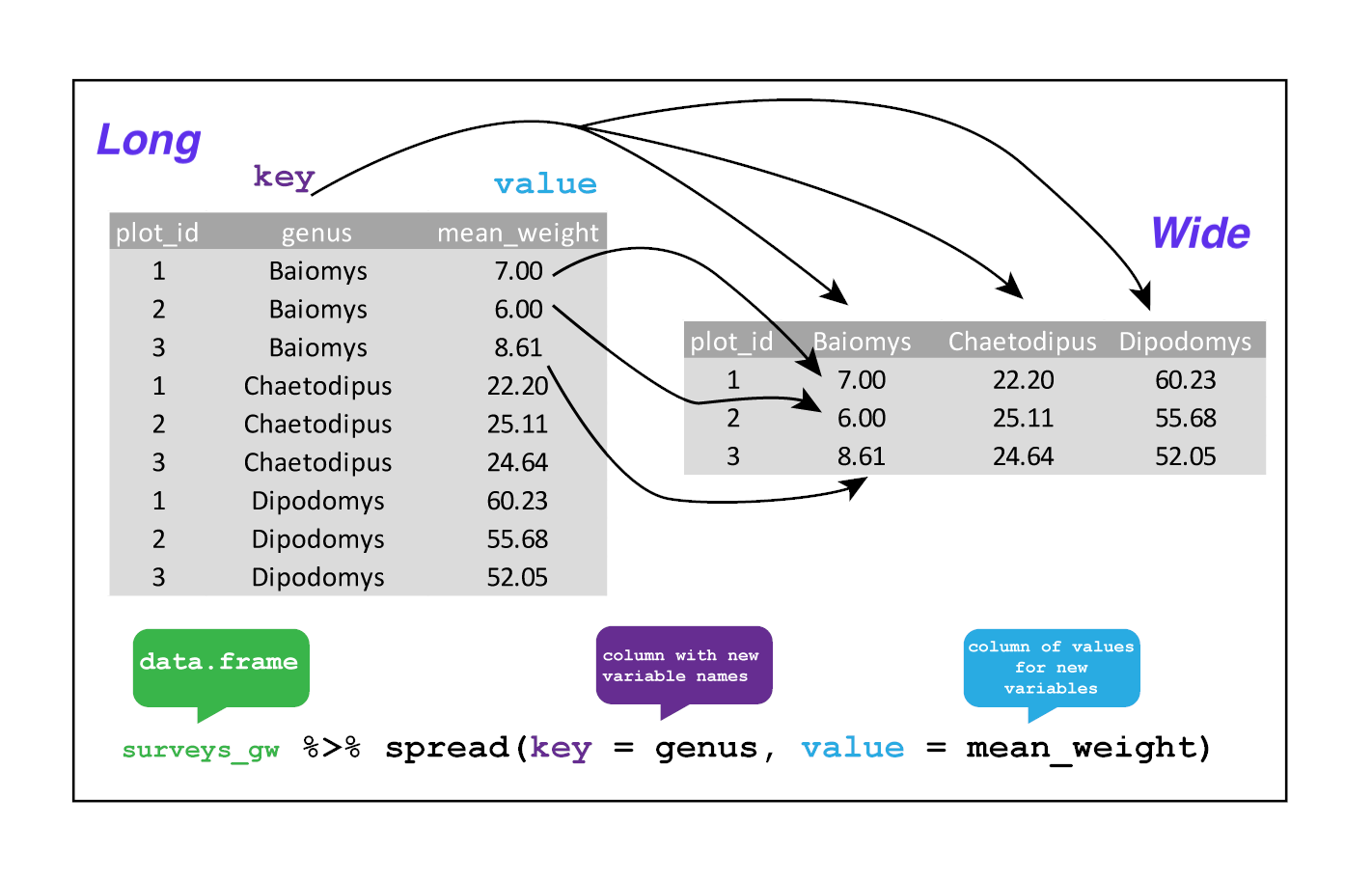
3.3.1 Comments
The comment character in R is
#, and anything in a script to the right of a#is disregarded by R. Leaving notes and clarifications in your scripts is beneficial. To remark or uncomment a paragraph in RStudio, select the lines you want to comment and hitCtrl + Shift + Con your keyboard at the same time. If you only want to comment out one line, place the cursor wherever on it (no need to select the entire line), then clickCtrl + Shift + C.Exercise
What are the values after each statement in the following?