Machine Learning Methods For Material Sciences

Machine Learning Fundamentals

next episode

Overview

Questions

What are the fundamental concepts in ML I can use in sklearn framewrok ?

How do I write documentation for my ML code?

How do I train and test ML models for material Sciences Problems?

Objectives

Gain an understanding of fundamental machine learning concepts relevant to material sciences.

Develop proficiency in optimizing data preprocessing techniques for machine learning tasks in Python.

Learn and apply best practices for training, evaluating, and interpreting machine learning models in the domain of material sciences.

Apply similarity metrics (e.g., cosine similarity) to quantify structural resemblance

Materials Properties Datasets

These datasets compute properties of various materials.

dc.molnet.load_bandgap : V2 dc.molnet.load_perovskite : V2 dc.molnet.load_mp_formation_energy : V2 dc.molnet.load_mp_metallicity : V2 [3] Lopez, Steven A., et al. “The Harvard organic photovoltaic dataset.” Scientific data 3.1 (2016): 1-7.

[4] Ramsundar, Bharath, et al. “Is multitask deep learning practical for pharma?.” Journal of chemical information and modeling 57.8 (2017): 2068-2076.

What is a Fingerprint?

Deep learning models almost always take arrays of numbers as their inputs. If we want to process molecules with them, we somehow need to represent each molecule as one or more arrays of numbers.

Many (but not all) types of models require their inputs to have a fixed size. This can be a challenge for molecules, since different molecules have different numbers of atoms. If we want to use these types of models, we somehow need to represent variable sized molecules with fixed sized arrays.

Fingerprints are designed to address these problems. A fingerprint is a fixed length array, where different elements indicate the presence of different features in the molecule. If two molecules have similar fingerprints, that indicates they contain many of the same features, and therefore will likely have similar chemistry.

DScribe

DScribe is a Python package for transforming atomic structures into fixed-size numerical fingerprints. These fingerprints are often called “descriptors” and they can be used in various tasks, including machine learning, visualization, similarity analysis, etc. The libary introduce the descriptor and demonstrate their basic call signature. We have also included several examples that should cover many of the use cases.

Coulomb Matrix
Sine matrix
Ewald sum matrix
Atom-centered Symmetry Functions
Smooth Overlap of Atomic Positions
Many-body Tensor Representation
Local Many-body Tensor Representation
Valle-Oganov descriptor

DScribe provides methods to transform atomic structures into fixed-size numeric vectors. These vectors are built in a way that they efficiently summarize the contents of the input structure. Such a transformation is very useful for various purposes, e.g.

Input for supervised machine learning models, e.g. regression.
Input for unsupervised machine learning models, e.g. clustering.
Visualizing and analyzing a local chemical environment.
Measuring similarity of structures or local structural sites. etc.

# https://doi.org/10.1016/j.cpc.2019.106949
#!pip install dscribe
import numpy as np
from ase.build import molecule
from dscribe.descriptors import SOAP, CoulombMatrix

# ========================================
# 1. Define Atomic Structures
# ========================================
print("Building molecular samples...")
samples = [
    molecule("H2O"),  # Water (3 atoms)
    molecule("NO2"),  # Nitrogen dioxide (3 atoms)
    molecule("CO2")   # Carbon dioxide (3 atoms)
]

# Print basic info
for i, mol in enumerate(samples):
    formula = mol.get_chemical_formula()
    atomic_numbers = mol.get_atomic_numbers()
    print(f"Sample {i}: {formula}, atoms = {len(mol)}, atomic numbers = {atomic_numbers}")

# ========================================
# 2. Setup Descriptors
# ========================================
print("\nSetting up descriptors...")

# Coulomb Matrix: Global molecular descriptor
cm_desc = CoulombMatrix(
    n_atoms_max=3,
    permutation="sorted_l2"  # Ensures consistent ordering
)

# SOAP: Local environment descriptor
soap_desc = SOAP(
    species=["H", "C", "N", "O"],  # All elements in the dataset
    r_cut=5.0,                     # Cutoff radius in Å
    n_max=8,                       # Number of radial basis functions
    l_max=6                        # Number of angular basis functions
)

# ========================================
# 3. Coulomb Matrix for Single and Multiple Systems
# ========================================
print("\n--- Computing Coulomb Matrices ---")

# Single molecule (H2O)
water = samples[0]
cm_single = cm_desc.create(water)
print(f"Coulomb Matrix (H2O) shape: {cm_single.shape}")
print(f"Coulomb Matrix (flattened): {cm_single}")

# Batch: All molecules
cm_batch = cm_desc.create(samples)
cm_batch_parallel = cm_desc.create(samples, n_jobs=2)

print(f"Batch Coulomb matrices shape: {cm_batch.shape}")        # (3, 9)
print(f"Parallel batch shape: {cm_batch_parallel.shape}")

# ========================================
# 4. SOAP Descriptors for Oxygen Atoms Only
# ========================================
print("\n--- Computing SOAP Descriptors for Oxygen Atoms ---")

# Find oxygen atom indices in each molecule
oxygen_indices = [np.where(mol.get_atomic_numbers() == 8)[0] for mol in samples]
print(f"Oxygen atom indices per molecule: {oxygen_indices}")

# Compute SOAP only for oxygen atoms
oxygen_soap_list = soap_desc.create(samples, oxygen_indices, n_jobs=2)

# Output is a list of arrays (variable number of centers per molecule)
print(f"SOAP output type: {type(oxygen_soap_list)}")
for i, soap_per_mol in enumerate(oxygen_soap_list):
    mol_formula = samples[i].get_chemical_formula()
    print(f"  Molecule {i} ({mol_formula}): {soap_per_mol.shape} SOAP vectors")

# Flatten into a single 2D array: (N_total_oxygens, n_features)
oxygen_soap_flat = np.vstack(oxygen_soap_list)
print(f"Flattened SOAP descriptors shape (all oxygen atoms): {oxygen_soap_flat.shape}")
# Example: (5, 3696) → 1 (H2O) + 2 (NO2) + 2 (CO2)

# ========================================
# 5. Compute SOAP Derivatives (w.r.t. Atomic Positions)
# ========================================
print("\n--- Computing SOAP Derivatives ---")

try:
    derivatives_list, descriptors_list = soap_desc.derivatives(
        samples,
        centers=oxygen_indices,
        return_descriptor=True,
        n_jobs=1  # Derivatives often work best with n_jobs=1
    )

    # 'derivatives_list' is a list: one entry per molecule, shape (n_centers, 3, n_features)
    print("SOAP derivatives computed successfully (returned as list).")
    print(f"Number of molecules in derivatives: {len(derivatives_list)}")
    for i, d in enumerate(derivatives_list):
        print(f"  Molecule {i}: derivative shape = {d.shape}")

except Exception as e:
    print(f"Error computing derivatives: {e}")

# ========================================
# 6. Final Summary
# ========================================
print("\n--- Summary ---")
print(f"Total molecules: {len(samples)}")
print(f"Coulomb Matrices: shape {cm_batch.shape} → used for global molecular representation")
print(f"SOAP (oxygen atoms): flattened to {oxygen_soap_flat.shape} → ready for machine learning")
if 'derivatives_list' in locals():
    total_deriv_centers = sum(d.shape[0] for d in derivatives_list)
    print(f"SOAP derivatives: {total_deriv_centers} centers total → useful for force prediction")
else:
    print("SOAP derivatives: not available")

The above example employs atomistic descriptors to generate machine-readable representations of small inorganic molecules—H₂O, NO₂, and CO₂—using the DScribe library. Two distinct types of descriptors are utilized: the Coulomb Matrix (CM) and the Smooth Overlap of Atomic Positions (SOAP). The CM provides a global, rotation- and permutation-invariant representation of each molecule, encoded as a fixed-size vector of dimension $ n_{\text{atoms}}^{\text{max}} \times n_{\text{atoms}}^{\text{max}} $, here flattened to a 9-dimensional vector after sorting by L2 norm to ensure consistency across configurations. This representation is suitable for regression tasks targeting global molecular properties such as total energy.

In contrast, the SOAP descriptor offers a local, chemically rich description of atomic environments, computed specifically for oxygen atoms across all structures. Due to the variable number of oxygen atoms per molecule (one in H₂O, two in NO₂ and CO₂), the resulting descriptors are structured as a list of arrays, later concatenated into a unified feature matrix of shape (5, 3696), where each row corresponds to an oxygen-centered environment and columns represent the high-dimensional SOAP basis expansion ($ n_{\text{max}} = 8 $, $ l_{\text{max}} = 6 $). This localized approach enables atom-centered machine learning models, including those predicting partial charges, chemical shifts, or reactivity.

Furthermore, analytical derivatives of the SOAP descriptor with respect to atomic positions are computed, enabling the prediction of forces in energy-conserving machine learning potentials. These derivatives are returned per center and per Cartesian direction, forming a hierarchical structure suitable for integration into gradient-based learning frameworks.

The use of parallelization via the n_jobs parameter demonstrates scalability for larger datasets. Overall, this work establishes a reproducible pipeline for generating physically meaningful descriptors from molecular geometries, forming a foundation for subsequent applications in quantum property prediction, potential energy surface construction, and interpretative analysis in computational chemistry and materials informatics.

Coulomb Matrix (CM)

Coulomb Matrix (CM) is a simple global descriptor which mimics the electrostatic interaction between nuclei. Coulomb matrix is calculated with the equation below.

\[M_{ij}^\mathrm{Coulomb} = \begin{cases} 0.5 Z_i^{2.4} & \text{for } i = j \\ \frac{Z_i Z_j}{R_{ij}} & \text{for } i \neq j \end{cases}\]

In the matrix above the first row corresponds to carbon (C) in methanol interacting with all the other atoms (columns 2-5) and itself (column 1). Likewise, the first column displays the same numbers, since the matrix is symmetric. Furthermore, the second row (column) corresponds to oxygen and the remaining rows (columns) correspond to hydrogen (H). Can you determine which one is which?

Since the Coulomb Matrix was published in 2012 more sophisticated descriptors have been developed. However, CM still does a reasonably good job when comparing molecules with each other. Apart from that, it can be understood intuitively and is a good introduction to descriptors.

from dscribe.descriptors import CoulombMatrix
from ase.build import molecule

# Define methanol molecule (example)
methanol = molecule("CH3OH")

# Setting up the CM descriptor with max atoms 6
cm = CoulombMatrix(n_atoms_max=6)

# Create CM output for methanol
cm_methanol = cm.create(methanol)
print("Coulomb matrix for methanol:\n", cm_methanol)

# Create output for multiple systems
samples = [molecule("H2O"), molecule("NO2"), molecule("CO2")]

# Serial creation
coulomb_matrices_serial = cm.create(samples)
print("Serial Coulomb matrices shape:", coulomb_matrices_serial.shape)

# Parallel creation using 2 jobs (if supported)
coulomb_matrices_parallel = cm.create(samples, n_jobs=2)
print("Parallel Coulomb matrices shape:", coulomb_matrices_parallel.shape)

# No sorting
cm_none = CoulombMatrix(n_atoms_max=6, permutation='none')
cm_methanol_none = cm_none.create(methanol)
print("\nChemical symbols:", methanol.get_chemical_symbols())
print("Coulomb matrix without sorting:\n", cm_methanol_none)

# Sort by Euclidean (L2) norm
cm_sorted = CoulombMatrix(n_atoms_max=6, permutation='sorted_l2')
cm_methanol_sorted = cm_sorted.create(methanol)
print("Coulomb matrix sorted by L2 norm:\n", cm_methanol_sorted)

# Random permutation
cm_random = CoulombMatrix(n_atoms_max=6, permutation='random', sigma=70, seed=None)
cm_methanol_random = cm_random.create(methanol)
print("Coulomb matrix with random permutation:\n", cm_methanol_random)

# Eigenspectrum
cm_eigen = CoulombMatrix(n_atoms_max=6, permutation='eigenspectrum')
cm_methanol_eigen = cm_eigen.create(methanol)
print("Eigenspectrum of Coulomb matrix:\n", cm_methanol_eigen)

Coulomb matrix for methanol:
 [73.51669472 33.73297539  8.24741496  3.96011613  3.808905    3.808905
 33.73297539 36.8581052   3.08170819  5.50690929  5.47078813  5.47078813
  8.24741496  3.08170819  0.5         0.35443545  0.42555057  0.42555057
  3.96011613  5.50690929  0.35443545  0.5         0.56354208  0.56354208
  3.808905    5.47078813  0.42555057  0.56354208  0.5         0.56068143
  3.808905    5.47078813  0.42555057  0.56354208  0.56068143  0.5       ]
Serial Coulomb matrices shape: (3, 36)
Parallel Coulomb matrices shape: (3, 36)

Chemical symbols: ['C', 'O', 'H', 'H', 'H', 'H']
Coulomb matrix without sorting:
 [36.8581052  33.73297539  5.50690929  3.08170819  5.47078813  5.47078813
 33.73297539 73.51669472  3.96011613  8.24741496  3.808905    3.808905
  5.50690929  3.96011613  0.5         0.35443545  0.56354208  0.56354208
  3.08170819  8.24741496  0.35443545  0.5         0.42555057  0.42555057
  5.47078813  3.808905    0.56354208  0.42555057  0.5         0.56068143
  5.47078813  3.808905    0.56354208  0.42555057  0.56068143  0.5       ]
Coulomb matrix sorted by L2 norm:
 [73.51669472 33.73297539  8.24741496  3.96011613  3.808905    3.808905
 33.73297539 36.8581052   3.08170819  5.50690929  5.47078813  5.47078813
  8.24741496  3.08170819  0.5         0.35443545  0.42555057  0.42555057
  3.96011613  5.50690929  0.35443545  0.5         0.56354208  0.56354208
  3.808905    5.47078813  0.42555057  0.56354208  0.5         0.56068143
  3.808905    5.47078813  0.42555057  0.56354208  0.56068143  0.5       ]
Coulomb matrix with random permutation:
 [ 0.5         0.56354208  3.96011613  5.50690929  0.35443545  0.56354208
  0.56354208  0.5         3.808905    5.47078813  0.42555057  0.56068143
  3.96011613  3.808905   73.51669472 33.73297539  8.24741496  3.808905
  5.50690929  5.47078813 33.73297539 36.8581052   3.08170819  5.47078813
  0.35443545  0.42555057  8.24741496  3.08170819  0.5         0.42555057
  0.56354208  0.56068143  3.808905    5.47078813  0.42555057  0.5       ]
Eigenspectrum of Coulomb matrix:
 [ 9.55802663e+01  1.81984422e+01 -8.84554212e-01 -4.08434021e-01
 -6.06814298e-02 -5.02389071e-02]

The descriptor is computed both for individual molecules and batches, with support for parallel computation via the n_jobs parameter to improve efficiency on multiple structures.

This approach exemplifies how molecular structure data can be systematically converted into machine-learning-ready descriptors while handling permutation symmetries and computational performance, facilitating tasks such as property prediction and molecular similarity analysis in cheminformatics and materials informatics.

invariance tests (translation, rotation, permutation)

Incorporating the invariance tests (translation, rotation, permutation) of the methanol molecule, as well as showing that the Coulomb Matrix descriptor is not designed for periodic systems (pbc set to True). The following code uses ASE methods to manipulate the molecule and demonstrates that the Coulomb matrix remains invariant or changes accordingly.

from dscribe.descriptors import CoulombMatrix
from ase.build import molecule
import numpy as np

# Build methanol molecule
methanol = molecule("CH3OH")

# Initialize Coulomb Matrix descriptor with permutation sorted by L2 norm (invariance)
cm = CoulombMatrix(n_atoms_max=6, permutation="sorted_l2")

# Original Coulomb matrix
cm_methanol = cm.create(methanol)
print("Original Coulomb matrix:")
print(cm_methanol)

# --- Invariance tests ---

# Translation: translate methanol by vector (5, 7, 9)
methanol_translated = methanol.copy()
methanol_translated.translate((5, 7, 9))
cm_methanol_translated = cm.create(methanol_translated)
print("\nCoulomb matrix after translation:")
print(cm_methanol_translated)

# Rotation: rotate methanol 90 degrees about the z-axis around origin
methanol_rotated = methanol.copy()
methanol_rotated.rotate(90, 'z', center=(0, 0, 0))
cm_methanol_rotated = cm.create(methanol_rotated)
print("\nCoulomb matrix after rotation:")
print(cm_methanol_rotated)

# Permutation: reverse atom order (upside down)
upside_down_methanol = methanol.copy()[::-1]
cm_methanol_permuted = cm.create(upside_down_methanol)
print("\nCoulomb matrix after permutation (atom reorder):")
print(cm_methanol_permuted)

# --- Periodic boundary conditions (not supported) ---

# Set periodic boundary conditions (PBC) and unit cell (not for molecules)
methanol_pbc = methanol.copy()
methanol_pbc.set_pbc([True, True, True])
methanol_pbc.set_cell([[10.0, 0.0, 0.0],
                       [0.0, 10.0, 0.0],
                       [0.0, 0.0, 10.0]])

cm_no_perm = CoulombMatrix(n_atoms_max=6)  # Default permutation

cm_methanol_pbc = cm_no_perm.create(methanol_pbc)
print("\nCoulomb matrix with periodic boundary conditions (not recommended):")
print(cm_methanol_pbc)

Original Coulomb matrix:
[73.51669472 33.73297539  8.24741496  3.96011613  3.808905    3.808905
73297539 36.8581052   3.08170819  5.50690929  5.47078813  5.47078813
24741496  3.08170819  0.5         0.35443545  0.42555057  0.42555057
96011613  5.50690929  0.35443545  0.5         0.56354208  0.56354208
808905    5.47078813  0.42555057  0.56354208  0.5         0.56068143
808905    5.47078813  0.42555057  0.56354208  0.56068143  0.5       ]

Coulomb matrix after translation:
[73.51669472 33.73297539  8.24741496  3.96011613  3.808905    3.808905
73297539 36.8581052   3.08170819  5.50690929  5.47078813  5.47078813
24741496  3.08170819  0.5         0.35443545  0.42555057  0.42555057
96011613  5.50690929  0.35443545  0.5         0.56354208  0.56354208
808905    5.47078813  0.42555057  0.56354208  0.5         0.56068143
808905    5.47078813  0.42555057  0.56354208  0.56068143  0.5       ]

Coulomb matrix after rotation:
[73.51669472 33.73297539  8.24741496  3.96011613  3.808905    3.808905
73297539 36.8581052   3.08170819  5.50690929  5.47078813  5.47078813
24741496  3.08170819  0.5         0.35443545  0.42555057  0.42555057
96011613  5.50690929  0.35443545  0.5         0.56354208  0.56354208
808905    5.47078813  0.42555057  0.56354208  0.5         0.56068143
808905    5.47078813  0.42555057  0.56354208  0.56068143  0.5       ]

Coulomb matrix after permutation (atom reorder):
[73.51669472 33.73297539  8.24741496  3.96011613  3.808905    3.808905
73297539 36.8581052   3.08170819  5.50690929  5.47078813  5.47078813
24741496  3.08170819  0.5         0.35443545  0.42555057  0.42555057
96011613  5.50690929  0.35443545  0.5         0.56354208  0.56354208
808905    5.47078813  0.42555057  0.56354208  0.5         0.56068143
808905    5.47078813  0.42555057  0.56354208  0.56068143  0.5       ]

Coulomb matrix with periodic boundary conditions (not recommended):
[73.51669472 33.73297539  8.24741496  3.96011613  3.808905    3.808905
73297539 36.8581052   3.08170819  5.50690929  5.47078813  5.47078813
24741496  3.08170819  0.5         0.35443545  0.42555057  0.42555057
96011613  5.50690929  0.35443545  0.5         0.56354208  0.56354208
808905    5.47078813  0.42555057  0.56354208  0.5         0.56068143
808905    5.47078813  0.42555057  0.56354208  0.56068143  0.5       ]

The sine matrix captures features of interacting atoms in a periodic system with a very low computational cost. The matrix elements are defined by

\[M_{ij}^\mathrm{sine} = \begin{cases} 0.5\, Z_i^{2.4} & i = j \\ \displaystyle \frac{Z_i Z_j}{\left| \mathbf{B} \cdot \sum_{k=x,y,z} \hat{\mathbf{e}}_k \sin^2\left( \pi \hat{\mathbf{e}}_k \mathbf{B}^{-1} \cdot (\mathbf{R}_i - \mathbf{R}_j) \right) \right|} & i \neq j \end{cases}\]

where:

$Z_i$: atomic number
$\mathbf{R}_i$: position of atom $ i $
$\mathbf{B}$: matrix of lattice vectors

It is part of the Crystal Metric Representations (CMR) family and is designed for fast, scalable materials comparison.

Exercise: Generating Sine Matrix Fingerprints

The Sine Matrix (SM) is a simple, computationally efficient fingerprint for crystalline solids that captures long-range atomic interactions in a translationally and rotationally invariant manner. It is particularly useful for high-throughput screening and similarity analysis in materials databases. In this exercise, you will:

Construct a set of common inorganic crystals using ASE.
Compute the Sine Matrix descriptor for each material using DScribe.
Explore the structure of the Sine Matrix: diagonal (self-term) vs. off-diagonal (interaction) elements.
Visualize the descriptor vectors (flattened matrices) using heatmaps and bar plots.
Compare fingerprints across different crystal structures (e.g., rocksalt vs. diamond).

This exercise focuses exclusively on fingerprint generation, not on property prediction or model training.

Solution

import numpy as np
import matplotlib.pyplot as plt
import seaborn as sns
from ase.build import bulk
from dscribe.descriptors import SineMatrix

# ========================================
# 1. Build Inorganic Crystal Structures
# ========================================
print("Building crystalline materials...\n")

# Note: 'cesium_chloride' not supported; using 'bcc' template
cscl = bulk("Cs", "bcc", a=4.12, cubic=True)
cscl.set_chemical_symbols(["Cs", "Cl"])  # Cs at (0,0,0), Cl at (0.5,0.5,0.5)

materials = [
    bulk("Si", "diamond", a=5.43),           # Diamond cubic
    bulk("NaCl", "rocksalt", a=5.64),        # Rocksalt
    cscl,                                    # CsCl structure (fixed)
    bulk("GaAs", "zincblende", a=5.65),      # Zincblende
    bulk("ZnO", "wurtzite", a=3.25, c=5.21)  # Wurtzite
]

names = ["Si", "NaCl", "CsCl", "GaAs", "ZnO"]

for i, name in enumerate(names):
    natoms = len(materials[i])
    formula = materials[i].get_chemical_formula()
    print(f"{name}: {formula}, atoms = {natoms}, structure = {materials[i].pbc}")

# ========================================
# 2. Setup Sine Matrix Descriptor
# ========================================
print("\nSetting up Sine Matrix descriptor...")

sm_desc = SineMatrix(
    n_atoms_max=8,           # Maximum number of atoms in unit cell
    permutation="none"       # Keep original atom order
)

# Compute Sine Matrix (output is always flattened in DScribe >=0.5)
fingerprints = sm_desc.create(materials)
print(f"Flattened fingerprint shape: {fingerprints.shape}")  # (n_samples, 64)

# Reshape to get matrix form: (n_samples, 8, 8)
sine_matrices = fingerprints.reshape(len(materials), 8, 8)
print(f"Sine Matrix output shape: {sine_matrices.shape}")     # (n_samples, 8, 8)

# ========================================
# 3. Analyze Sine Matrix Structure
# ========================================
for i, name in enumerate(names):
    M = sine_matrices[i]  # (8, 8)
    n_actual = len(materials[i])

    print(f"\n--- {name} Sine Matrix Summary ---")
    diag_mean = np.diag(M)[:n_actual].mean()
    off_diag_vals = M[~np.eye(M.shape[0], dtype=bool)]  # Off-diagonal elements only
    off_diag_mean = off_diag_vals.mean()
    print(f"  Diagonal (self-interaction) mean: {diag_mean:.3f}")
    print(f"  Off-diagonal (interaction) mean: {off_diag_mean:.3f}")
    print(f"  Max value: {M.max():.3f}, Min value: {M.min():.3f}")

# ========================================
# 4. Visualize Sine Matrices
# ========================================
fig, axes = plt.subplots(2, 3, figsize=(12, 8))
axes = axes.flatten()

for i, name in enumerate(names):
    M = sine_matrices[i]
    sns.heatmap(
        M,
        ax=axes[i],
        cmap="Blues",
        cbar=True,
        square=True,
        cbar_kws={"shrink": 0.8}
    )
    axes[i].set_title(f"{name} Sine Matrix")

# Remove last subplot
fig.delaxes(axes[-1])

plt.suptitle("Sine Matrix Fingerprints for Crystalline Materials", fontsize=14)
plt.tight_layout()
plt.savefig("sine_matrix_heatmaps.png", dpi=150)
plt.show()

# ========================================
# 5. Compare Flattened Fingerprints
# ========================================
plt.figure(figsize=(10, 6))
x_pos = np.arange(fingerprints.shape[1])  # Feature index

colors = ["tab:blue", "tab:orange", "tab:green", "tab:red", "tab:purple"]
for i, name in enumerate(names):
    plt.plot(x_pos, fingerprints[i], color=colors[i], label=name, linewidth=1.5, alpha=0.8)

plt.xlabel("Feature Index (Flattened Sine Matrix)", fontsize=12)
plt.ylabel("Descriptor Value", fontsize=12)
plt.title("Comparison of Flattened Sine Matrix Fingerprints", fontsize=13)
plt.legend()
plt.grid(True, alpha=0.3)
plt.tight_layout()
plt.savefig("sine_matrix_fingerprints.png", dpi=150)
plt.show()

# ========================================
# 6. Compute Pairwise Similarity
# ========================================
print("\nPairwise Cosine Similarity Between Fingerprints:")
from sklearn.metrics.pairwise import cosine_similarity

sim_matrix = cosine_similarity(fingerprints)
np.set_printoptions(precision=3, suppress=True)
print("Similarity matrix:")
print(sim_matrix)

# Heatmap of similarity
plt.figure(figsize=(6, 5))
sns.heatmap(
    sim_matrix,
    annot=True,
    xticklabels=names,
    yticklabels=names,
    cmap="Reds",
    vmin=0.5, vmax=1.0
)
plt.title("Cosine Similarity Between Sine Matrix Fingerprints")
plt.tight_layout()
plt.savefig("sine_matrix_similarity.png", dpi=150)
plt.show()

Ewald Sum Matrix for Periodic Crystals

The Ewald Sum Matrix (ESM) extends the concept of the Coulomb matrix to periodic systems by modeling the full electrostatic interaction between atomic cores in a crystal, including long-range Coulomb forces and a neutralizing background. It is particularly useful for capturing charge distribution effects and electrostatic stability in ionic materials.

Exercise: Ewald Sum Matrix

The Ewald Sum Matrix (ESM) extends the Coulomb matrix to periodic systems by modeling the full electrostatic interaction between atomic cores in a crystal, including long-range Coulomb forces and a neutralizing background. It is particularly useful for capturing charge distribution effects and electrostatic stability in ionic materials.

In this exercise, you will:

Construct common crystals (NaCl, Al, Fe) using ASE.
Set up the Ewald Sum Matrix descriptor using DScribe.
Compute ESMs for single and multiple systems (serial and parallel).
Explore how convergence parameters affect accuracy.
Estimate the total electrostatic energy of a crystal from the ESM.

This exercise focuses on descriptor generation and physical interpretation, not on machine learning.

Solution

# 1. Import and Setup
import numpy as np
import scipy.constants
import math
from ase.build import bulk
from dscribe.descriptors import EwaldSumMatrix

print("Setting up systems and descriptor...\n")

# Create NaCl crystal
nacl = bulk("NaCl", "rocksalt", a=5.64)
al = bulk("Al", "fcc", a=4.046)
fe = bulk("Fe", "bcc", a=2.856)

# List of samples for batch processing
samples = [nacl, al, fe]
names = ["NaCl", "Al", "Fe"]

for name, atoms in zip(names, samples):
    formula = atoms.get_chemical_formula()
    print(f"{name}: {formula}, atoms = {len(atoms)}, cell = {atoms.cell.lengths()[0]:.3f} Å")

# 2. Setup Ewald Sum Matrix Descriptor
esm = EwaldSumMatrix(
    n_atoms_max=6
)

# 3. Create ESM for Single System
print("\nCreating ESM for NaCl...")
nacl_ewald = esm.create(nacl, flatten=False)
print(f"NaCl ESM shape: {nacl_ewald.shape}")

# 4. Create ESM for Multiple Systems
print("\nCreating ESM for multiple systems (serial)...")
ewald_matrices = esm.create(samples, flatten=False)  # Serial
print(f"Batch ESM shape: {ewald_matrices.shape}")

print("\nCreating ESM in parallel (n_jobs=2)...")
ewald_matrices_parallel = esm.create(samples, n_jobs=2, flatten=False)

# 5. Vary Accuracy via Alpha (Convergence Parameter)
print("\nTesting different convergence parameters (alpha)...")
ewald_1 = esm.create(nacl, alpha=2.0)  # Lower accuracy
ewald_2 = esm.create(nacl, alpha=4.0)  # Higher accuracy
print(f"Low-alpha fingerprint norm: {np.linalg.norm(ewald_1):.2f}")
print(f"High-alpha fingerprint norm: {np.linalg.norm(ewald_2):.2f}")

# 6. Calculate Total Electrostatic Energy
print("\nCalculating total electrostatic energy for Al (example)...")
# Use a symmetric system (Al is neutral, Z=3)
ems = EwaldSumMatrix(
    n_atoms_max=2,           # FCC Al has 1 atom conventional → expand or use 2-atom cell
    permutation="none",
    sigma=1.0,
    alpha=3.0
)

# Use 2-atom cell to see interactions
al_expanded = al * (2, 1, 1)  # Now has 2 atoms
ems_out_flat = ems.create(al_expanded)
ems_out = ems.unflatten(ems_out_flat)[0]  # Extract first (only) system

# Total electrostatic energy ≈ sum of all entries divided by 2 (each interaction counted twice)
# But: ESM includes self-energy and interaction terms
total_energy = ems_out.sum() / 2  # Each pair counted twice; self-terms once

# Convert from atomic units (e²/Å) to eV
conversion = 1e10 * scipy.constants.e / (4 * math.pi * scipy.constants.epsilon_0)
total_energy_eV = total_energy * conversion

print(f"Total electrostatic energy (approx): {total_energy_eV:.4f} eV")

# 7. Summary
print("\n💡 Key Points:")
print("  • ESM captures long-range electrostatics in periodic systems.")
print("  • Use 'alpha' to control real/reciprocal space balance.")
print("  • Parallelization via 'n_jobs' speeds up batch processing.")
print("  • Total energy can be estimated from sum of ESM entries (with care).")

Machine Learning

The Smooth Overlap of Atomic Positions (SOAP) descriptor encodes the local atomic environment by representing the neighboring atomic density around each atom using expansions in spherical harmonics and radial basis functions within a cutoff radius. Parameters such as the cutoff radius, number of radial basis functions, maximum degree of spherical harmonics, and Gaussian smearing width control the descriptor’s resolution and size. The DScribe library efficiently computes these SOAP descriptors along with their derivatives with respect to atomic positions, enabling force predictions.

In machine learning models, the SOAP descriptor $\mathbf{D}$ serves as the input to predict system properties like total energy through a function $f(\mathbf{D})$. The predicted forces on atom $i$, denoted $\hat{\mathbf{F}}_i$, are obtained as the negative gradient of the predicted energy with respect to that atom’s position $\mathbf{r}_i$, expressed as:

\[\hat{\mathbf{F}}_i = - \nabla_{\mathbf{r}_i} f(\mathbf{D}) = - \nabla_{\mathbf{D}} f \cdot \nabla_{\mathbf{r}_i} \mathbf{D}\]

Here, $\nabla_{\mathbf{D}} f$ is the derivative of the model output with respect to the descriptor, which neural networks provide analytically, and $\nabla_{\mathbf{r}_i} \mathbf{D}$ is the Jacobian matrix of descriptor derivatives with respect to atomic coordinates, given by DScribe for SOAP. This equation expands as the dot product between the row vector of partial derivatives of the energy with respect to descriptor components and the matrix of derivatives of each descriptor component with respect to spatial coordinates:

\[\hat{\mathbf{F}}_i = - \begin{bmatrix} \frac{\partial f}{\partial D_1} & \frac{\partial f}{\partial D_2} & \dots \end{bmatrix} \begin{bmatrix} \frac{\partial D_1}{\partial x_i} & \frac{\partial D_1}{\partial y_i} & \frac{\partial D_1}{\partial z_i} \\ \frac{\partial D_2}{\partial x_i} & \frac{\partial D_2}{\partial y_i} & \frac{\partial D_2}{\partial z_i} \\ \vdots & \vdots & \vdots \\ \end{bmatrix}\]

DScribe organizes these derivatives such that the last dimension corresponds to descriptor features, optimizing performance in row-major data formats such as NumPy or C/C++ by making the dot product over the fastest-varying dimension more efficient, although this layout can be adapted as needed.

Training requires a dataset composed of feature vectors $\mathbf{D}$, their derivatives $\nabla_{\mathbf{r}} \mathbf{D}$, as well as reference energies $E$ and forces $\mathbf{F}$. The loss function is formed by summing the mean squared errors (MSE) of energy and force predictions, each scaled by the inverse variance of the respective quantities in the training data to balance their contribution:

\[\text{Loss} = \frac{1}{\sigma_E^2} \mathrm{MSE}(E, \hat{E}) + \frac{1}{\sigma_F^2} \mathrm{MSE}(\mathbf{F}, \hat{\mathbf{F}})\]

This ensures the model learns to predict both energies and forces effectively. Together, these components form a pipeline where SOAP descriptors combined with neural networks and analytic derivatives enable accurate and efficient prediction of atomic energies and forces for molecular and materials simulations.

Dataset preparation

This script prepare a training dataset of Lennard-Jones energies and forces for a simple two-atom system with varying interatomic distances. It uses the SOAP descriptor to characterize atomic environments and includes computation of analytical derivatives needed for force prediction.

import numpy as np
import ase
from ase.calculators.lj import LennardJones
import matplotlib.pyplot as plt
from dscribe.descriptors import SOAP

# Initialize SOAP descriptor
soap = SOAP(
    species=["H"],
    periodic=False,
    r_cut=5.0,
    sigma=0.5,
    n_max=3,
    l_max=0,
)

# Generate data for 200 samples with distances from 2.5 to 5.0 Å
n_samples = 200
traj = []
n_atoms = 2
energies = np.zeros(n_samples)
forces = np.zeros((n_samples, n_atoms, 3))
distances = np.linspace(2.5, 5.0, n_samples)

for i, d in enumerate(distances):
    # Create two hydrogen atoms separated by distance d along x-axis
    atoms = ase.Atoms('HH', positions=[[-0.5 * d, 0, 0], [0.5 * d, 0, 0]])
    atoms.set_calculator(LennardJones(epsilon=1.0, sigma=2.9))
    atoms.cal = cal
    traj.append(atoms)
    
    energies[i] = atoms.get_total_energy()
    forces[i] = atoms.get_forces()

# Validate energies by plotting against distance
plt.figure(figsize=(8,5))
plt.plot(distances, energies, label="Energy")
plt.xlabel("Distance (Å)")
plt.ylabel("Energy (eV)")
plt.title("Lennard-Jones Energies vs Distance")
plt.grid(True)
plt.savefig("Lennard-Jones_Energies_vs_Distance.png")
plt.show()

# Compute SOAP descriptors and their analytical derivatives with respect to atomic positions
# The center is fixed at the midpoint between the two atoms
derivatives, descriptors = soap.derivatives(
    traj,
    centers=[[[0, 0, 0]]] * n_samples,
    method="analytical"
)

# Save datasets for training
np.save("r.npy", distances)
np.save("E.npy", energies)
np.save("D.npy", descriptors)
np.save("dD_dr.npy", derivatives)
np.save("F.npy", forces)

The energies obtained from the Lennard-Jones two-atom system as a function of interatomic distance typically exhibit a characteristic curve, where the energy decreases sharply as the atoms approach each other, reaches a minimum at the equilibrium bond length, and then rises gradually as the atoms move further apart. This shape reflects the balance between attractive and repulsive forces in the Lennard-Jones potential.

In the plotted energy vs. distance graph, you will see a smooth curve starting at a higher energy around shorter distances (due to strong repulsion), dipping to a minimum energy near the equilibrium separation (around 3.0 Å for the parameters used), and then slowly increasing as the distance increases (weaker attraction).

This energy profile validates the dataset by demonstrating the physically meaningful behavior of the system’s interaction potential, which the machine learning model aims to learn and reproduce.

import numpy as np
from sklearn.preprocessing import StandardScaler
from sklearn.model_selection import train_test_split
from sklearn.ensemble import RandomForestRegressor
from sklearn.svm import SVR
from sklearn.metrics import mean_absolute_error

# Load dataset (numpy arrays)
D_numpy = np.load("D.npy")[:, 0, :]          # SOAP descriptor: one center per sample
E_numpy = np.load("E.npy")                    # Energies, shape (n_samples,)
F_numpy = np.load("F.npy")                    # Forces (not used here)
dD_dr_numpy = np.load("dD_dr.npy")            # Descriptor derivatives (not used here)
r_numpy = np.load("r.npy")                    # Distances (optional)

# Select training subset (e.g., 30 points evenly spaced)
n_train = 30
idx = np.linspace(0, len(r_numpy) - 1, n_train).astype(int)

D_train_full = D_numpy[idx]
E_train_full = E_numpy[idx]

# Scale features for better model training
scaler = StandardScaler()
D_train_full_scaled = scaler.fit_transform(D_train_full)
D_numpy_scaled = scaler.transform(D_numpy)

# Optional split train/validation (not mandatory for random forest or SVM)
# Here we use all training points directly for simplicity

# -------------------
# Random Forest Model
# -------------------
rf_model = RandomForestRegressor(n_estimators=100, random_state=7)
rf_model.fit(D_train_full_scaled, E_train_full)

# Predict energies on full dataset
E_pred_rf = rf_model.predict(D_numpy_scaled)

# Compute mean absolute error on full dataset
mae_rf = mean_absolute_error(E_pred_rf, E_numpy)
print(f"Random Forest Energy Prediction MAE: {mae_rf:.4f} eV")

# -------------------
# Support Vector Machine Model
# -------------------
svm_model = SVR(kernel='rbf', C=10.0, gamma='scale')
svm_model.fit(D_train_full_scaled, E_train_full)

# Predict energies on full dataset
E_pred_svm = svm_model.predict(D_numpy_scaled)

# Compute MAE for SVM
mae_svm = mean_absolute_error(E_pred_svm, E_numpy)
print(f"SVM Energy Prediction MAE: {mae_svm:.4f} eV")

Random Forest Energy Prediction MAE: 0.0830 eV
SVM Energy Prediction MAE: 0.0970 eV

Exercise: Predicting Atomic Forces with Random Forest and SVR

Machine learning models can predict atomic forces — essential for molecular dynamics, geometry optimization, and interatomic potential development. In this exercise, you will:

Generate a dataset of H₂ dimer configurations using the Lennard-Jones potential.
Compute SOAP descriptors for each atom in the system.
Train two models — Random Forest (RF) and Support Vector Regression (SVR) — using MultiOutputRegressor to predict 3D atomic forces.
Evaluate performance using Mean Absolute Error (MAE).
Understand how descriptors and regression strategies enable force learning.

This exercise focuses on force prediction, a core component of machine-learned force fields, and demonstrates the use of multi-output regression for vector-valued targets.

Solution

# 1. Import Libraries and Generate Data
import numpy as np
import ase
from ase.calculators.lj import LennardJones
from dscribe.descriptors import SOAP

print("Generating H₂ dimer dataset with Lennard-Jones forces...\n")
# Initialize SOAP descriptor
soap = SOAP(
    species=["H"],
    periodic=False,
   r_cut=5.0,
    sigma=0.5,
    n_max=3,
    l_max=0,
)
# Generate 200 samples: H₂ dimer at varying distances
n_samples = 200
traj = []
n_atoms = 2
energies = np.zeros(n_samples)
forces = np.zeros((n_samples, n_atoms, 3))  # Shape: (200, 2, 3)
distances = np.linspace(2.5, 5.0, n_samples)

for i, d in enumerate(distances):
    atoms = ase.Atoms('HH', positions=[[-0.5 * d, 0, 0], [0.5 * d, 0, 0]])
    calc = LennardJones(epsilon=1.0, sigma=2.9)
    atoms.calc = calc
    traj.append(atoms)
    energies[i] = atoms.get_total_energy()
    forces[i] = atoms.get_forces()

# Reshape forces for ML: (n_samples * n_atoms, 3)
forces_flat = forces.reshape(-1, 3)
print(f"Generated {n_samples} configurations with {n_atoms} atoms each.")
print(f"Force data shape (flattened): {forces_flat.shape}")
# 2. Compute SOAP Descriptors
print("\nComputing SOAP descriptors...")
centers = [[[0, 0, 0]]] * n_samples  # One center per system
descriptors = soap.create(traj, centers=centers)  # Shape: (200, 1, 6)
D = descriptors.squeeze(axis=1)  # Remove singleton dim → (200, 6)

# Repeat each descriptor for both atoms
D_repeated = np.repeat(D, n_atoms, axis=0)  # (200, 6) → (400, 6)
print(f"SOAP descriptor shape (repeated): {D_repeated.shape}")

# 3. Train-Test Split and Scaling
from sklearn.model_selection import train_test_split
from sklearn.preprocessing import StandardScaler

X_train, X_test, y_train, y_test = train_test_split(
    D_repeated, forces_flat, test_size=0.2, random_state=7
)

scaler = StandardScaler()
X_train_scaled = scaler.fit_transform(X_train)
X_test_scaled = scaler.transform(X_test)

# 4. Random Forest Model for Force Prediction
print("\nTraining Random Forest model on forces...")
from sklearn.ensemble import RandomForestRegressor
from sklearn.multioutput import MultiOutputRegressor
from sklearn.metrics import mean_absolute_error

rf_base = RandomForestRegressor(n_estimators=100, random_state=7)
rf_model = MultiOutputRegressor(rf_base)
rf_model.fit(X_train_scaled, y_train)

y_pred_rf = rf_model.predict(X_test_scaled)
mae_rf = mean_absolute_error(y_test, y_pred_rf)
print(f"Random Forest MAE (force): {mae_rf:.4f} eV/Å")

# 5. SVR Model for Force Prediction
print("\nTraining SVR model on forces...")
from sklearn.svm import SVR

svr_base = SVR(kernel='rbf', C=10.0, gamma='scale')
svr_model = MultiOutputRegressor(svr_base)
svr_model.fit(X_train_scaled, y_train)

y_pred_svr = svr_model.predict(X_test_scaled)
mae_svr = mean_absolute_error(y_test, y_pred_svr)
print(f"SVR MAE (force): {mae_svr:.4f} eV/Å")

Band Gap

Predicting band gaps using machine learning (ML) is a cutting-edge approach that enables fast and accurate estimation of a material’s electronic band gap—a key property influencing its electronic and optical behavior. ML models leverage extensive material databases and elemental descriptors to predict band gaps efficiently, overcoming the high computational costs and limitations of traditional methods like density functional theory (DFT). By training on known band gap data, ML models such as support vector regression, random forests, and gradient boosting can capture complex relationships between composition and band gap, accelerating the discovery of new materials with desired electronic properties. Additionally, some ML techniques offer interpretable models that provide insight into the physical factors affecting band gaps, making ML a powerful tool in materials science for band gap prediction and material design.

Getting the dataset

In this section, we demonstrate how to retrieve data on stable binary compounds from the Materials Project database using its API. By specifying criteria such as the number of elements and stability (energy above hull), we extract key material properties including chemical formula, symmetry, energy per atom, volume, and magnetization. The retrieved data is organized into a structured pandas DataFrame for easy analysis and further processing. This approach enables efficient access to high-quality materials data for research and machine learning applications.

from mp_api.client import MPRester
import pandas as pd
api_key = 'your_api_key'
fields = [
    "material_id", "formula_pretty", "symmetry",
    "nsites", "energy_per_atom", "volume",
    "energy_above_hull", "total_magnetization"
]

with MPRester(api_key) as mpr:
    docs = mpr.materials.summary.search(
        num_elements=[2, 2],                 
        energy_above_hull=(0, 0.001),        
        fields=fields
    )

records = []
for doc in docs:
    row = {
        "material_id": doc.material_id,
        "formula": doc.formula_pretty,
        "num_sites": doc.nsites,
        "energy_per_atom": doc.energy_per_atom,
        "volume": doc.volume,
        "energy_above_hull": doc.energy_above_hull,
        "total_magnetization": doc.total_magnetization
    }
    if doc.symmetry:
        row["spacegroup_number"] = doc.symmetry.number
        row["crystal_system"] = doc.symmetry.crystal_system   
    records.append(row)

df = pd.DataFrame(records)

print("Stable binary compounds count", len(df))
print(df.head())

Retrieving SummaryDoc documents: 100%|█| 5500/5500 [00:03<00:00, 1771.
Stable binary compounds count 5500
  material_id formula  num_sites  energy_per_atom       volume  \
  mp-11107   Ac2O3          5        -8.354915    91.511224   
  mp-32800   Ac2S3         40       -34.768478  1118.407852   
 mp-985305   Ac3In          8       -57.372981   309.226331   
 mp-985506   Ac3Tl          8       -64.936750   309.225189   
 mp-866199    AcAg          2       -45.267835    61.529375   

   energy_above_hull  total_magnetization  spacegroup_number crystal_system  
              0.0         0.000000e+00                164       Trigonal  
              0.0         0.000000e+00                122     Tetragonal  
              0.0         1.642045e+00                194      Hexagonal  
              0.0         3.199100e-03                194      Hexagonal  
              0.0         6.000000e-07                221          Cubic  

The result shows successful retrieval of data for 5,500 stable binary compounds from the Materials Project database. The extracted dataset includes key information such as material ID, chemical formula, number of atomic sites, energy per atom, volume, energy above hull (indicating stability), total magnetization, space group number, and crystal system. The preview of the dataset reveals a diverse set of compounds with a range of structural symmetries and electronic properties, providing a rich resource for further materials analysis and modeling.

Data Augmentation

In this section, we augment experimental band gap datasets by integrating them with structural and energetic data obtained from the Materials Project database. We retrieve stable compounds with 2 to 4 elements and combine these with multiple experimental band gap datasets to create a unified dataset. This merged dataset includes both experimental band gap values and corresponding material properties, facilitating more comprehensive analyses and model training.

from mp_api.client import MPRester
import pandas as pd
from matminer.datasets import load_dataset

api_key = "FAOXV20YqTT2edzIRotOaC2ayHn10cDT"

# query stable compounds with nelements = 2,3,4
fields = [
    "material_id", "formula_pretty", "symmetry",
    "nsites", "energy_per_atom", "volume",
    "energy_above_hull", "total_magnetization"
]

with MPRester(api_key) as mpr:
    docs = mpr.materials.summary.search(
        num_elements=[2, 4],    # range inclusive [2,4]
        energy_above_hull=(0, 0.001),
        fields=fields
    )

records = []
for doc in docs:
    row = {
        "material_id": doc.material_id,
        "formula": doc.formula_pretty,
        "num_sites": doc.nsites,
        "energy_per_atom": doc.energy_per_atom,
        "volume": doc.volume,
        "energy_above_hull": doc.energy_above_hull,
        "total_magnetization": doc.total_magnetization
    }
    if doc.symmetry:
        row["spacegroup_number"] = doc.symmetry.number
        row["crystal_system"] = doc.symmetry.crystal_system
    records.append(row)

df1 = pd.DataFrame(records)
print("Stable compounds (2–4 elements)", len(df1))
print(df1.head())

# ---- experimental band gap datasets ----
df2 = load_dataset("matbench_expt_gap")
df2 = df2.rename(columns={"composition": "formula", "gap expt": "gap_expt"})
df2 = df2[["formula", "gap_expt"]]

df3 = load_dataset("expt_gap")
df3 = df3.rename(columns={"formula": "formula", "gap expt": "gap_expt"})
df3 = df3[["formula", "gap_expt"]]

# union of experimental datasets
df4 = pd.concat([df2, df3], ignore_index=True)
df4 = df4[df4["gap_expt"] > 0].drop_duplicates("formula")
print("Experimental band gap entries", len(df4))
print(df4.head())

# ---- merge DFT structural features with experimental gaps ----
df = pd.merge(df1, df4, on="formula", how="inner")
df = df.drop_duplicates("formula", keep="first")

print("Final merged dataset", len(df))
print(df.head())

Retrieving SummaryDoc documents: 100%|██████████| 33972/33972 [00:15<00:00, 2261.30it/s]
Stable compounds (2–4 elements) 33972
  material_id  formula  num_sites  energy_per_atom      volume  \
mp-1183076  Ac2AgPb          4       -54.209271  134.563097   
mp-1183086  Ac2CdHg          4       -52.120621  133.072641   
 mp-862786  Ac2CuGe          4       -40.884684  113.979079   
 mp-861883  Ac2CuIr          4       -50.462576  104.095515   
 mp-867241  Ac2GePd          4        -5.176522  114.834178   

   energy_above_hull  total_magnetization  spacegroup_number crystal_system  
              0.0             0.910605                225          Cubic  
              0.0             0.628202                225          Cubic  
              0.0             0.001071                225          Cubic  
              0.0             0.000169                225          Cubic  
              0.0             0.000001                225          Cubic
Experimental band gap entries 3651
             formula  gap_expt
 Ag0.5Ge1Pb1.75S4      1.83
Ag0.5Ge1Pb1.75Se4      1.51
          Ag2GeS3      1.98
         Ag2GeSe3      0.90
          Ag2HgI4      2.47
Final merged dataset 1050
  material_id   formula  num_sites  energy_per_atom      volume  \
   mp-9900   Ag2GeS3         12        -4.253843  267.880017   
mp-1096802  Ag2GeSe3         12        -3.890180  309.160842   
  mp-23485   Ag2HgI4          7        -2.239734  266.737075   
    mp-353      Ag2O          6        -3.860246  107.442223   
mp-2018369      Ag2S         12       -17.033431  245.557534   

   energy_above_hull  total_magnetization  spacegroup_number crystal_system  \
         0.000000                  0.0                 36   Orthorhombic   
         0.000986                  0.0                 36   Orthorhombic   
         0.000000                  0.0                 82     Tetragonal   
         0.000000                  0.0                224          Cubic   
         0.000207                  0.0                 14     Monoclinic   

   gap_expt  
    1.98  
    0.90  
    2.47  
    1.50  
    1.23  

The results show the successful retrieval of 33,972 stable compounds with 2 to 4 elements from the Materials Project database. Additionally, 3,651 experimental band gap entries were obtained from multiple datasets. After merging these datasets based on the formula, a final unified dataset of 1,050 compounds was created. This merged dataset combines theoretical material properties (such as energy per atom, volume, and crystal symmetry) with experimentally measured band gap values, providing a valuable and comprehensive resource for material analysis and predictive modeling. The sample data illustrates a variety of compounds with detailed structural and electronic features alongside their experimental band gaps.

Feature engineering

In this step, we perform feature engineering on the dataset by extracting additional material descriptors from the chemical composition using the pymatgen and matminer libraries. Specifically, we convert the formula strings into Composition objects and apply the AtomicOrbitals featurizer to compute features related to atomic orbital characteristics. These new features enrich the dataset with meaningful chemical information that can improve the accuracy and interpretability of machine learning models for predicting band gaps. Missing values are removed to ensure data quality before further analysis

from pymatgen.core import Composition
from matminer.featurizers.composition import ElementProperty,AtomicOrbitals
df['composition'] = df.formula.map(lambda x: Composition(x))
df = df.dropna(axis=0)
df = AtomicOrbitals().featurize_dataframe(df, 
                                              'composition', 
                                              ignore_errors=True,
                                              return_errors=False)
(df[df.gap_AO > 0]).head()
df.head()

AtomicOrbitals: 100%|██████████| 1050/1050 [00:12<00:00, 84.01it/s] 
material_id	formula	num_sites	energy_per_atom	volume	energy_above_hull	total_magnetization	spacegroup_number	crystal_system	gap_expt	composition	HOMO_character	HOMO_element	HOMO_energy	LUMO_character	LUMO_element	LUMO_energy	gap_AO
mp-9900	Ag2GeS3	12	-4.253843	267.880017	0.000000	0.0	36	Orthorhombic	1.98	(Ag, Ge, S)	p	S	-0.261676	p	S	-0.261676	0.000000
mp-1096802	Ag2GeSe3	12	-3.890180	309.160842	0.000986	0.0	36	Orthorhombic	0.90	(Ag, Ge, Se)	p	Se	-0.245806	p	Se	-0.245806	0.000000
mp-23485	Ag2HgI4	7	-2.239734	266.737075	0.000000	0.0	82	Tetragonal	2.47	(Ag, Hg, I)	p	I	-0.267904	s	Hg	-0.205137	0.062767
mp-353	Ag2O	6	-3.860246	107.442223	0.000000	0.0	224	Cubic	1.50	(Ag, O)	d	Ag	-0.298706	s	Ag	-0.157407	0.141299
mp-2018369	Ag2S	12	-17.033431	245.557534	0.000207	0.0	

The results show that the AtomicOrbitals featurizer successfully generated atomic orbital-related features for all 1,050 entries in the dataset. These features include information about the highest occupied molecular orbital (HOMO) and lowest unoccupied molecular orbital (LUMO) characters, elements, and energies, as well as the calculated band gap based on atomic orbital data (gap_AO). The dataset now contains enhanced chemical descriptors such as orbital types (e.g., s, p, d), corresponding elements, and orbital energy levels, which provide deeper insight into the electronic structure of materials and can improve predictive modeling of their band gaps. The feature engineering process completed efficiently with comprehensive coverage across all materials.

Preprocessing features

In this step, we preprocess the atomic orbital character features by converting categorical orbital labels (such as s, p, d, f) into a consistent numeric format. This mapping standardizes the data, making it suitable for machine learning algorithms that require numerical inputs. Unknown or missing values are preserved as NaN to avoid incorrect data transformation, ensuring clean and reliable feature representation for model training.

# define consistent mapping
homo_lomo_mapper = {
    "s": 1,
    "p": 2,
    "d": 3,
    "f": 4,
}

# map to numeric, keep NaN for unknowns
df["HOMO_character"] = df["HOMO_character"].astype(str).str.strip().str.lower()
df["LUMO_character"] = df["LUMO_character"].astype(str).str.strip().str.lower()
df["HOMO_character"] = df["HOMO_character"].map(homo_lomo_mapper)
df["LUMO_character"] = df["LUMO_character"].map(homo_lomo_mapper)
df.head()

material_id	formula	num_sites	energy_per_atom	volume	energy_above_hull	total_magnetization	spacegroup_number	crystal_system	gap_expt	composition	HOMO_character	HOMO_element	HOMO_energy	LUMO_character	LUMO_element	LUMO_energy	gap_AO
mp-9900	Ag2GeS3	12	-4.253843	267.880017	0.000000	0.0	36	Orthorhombic	1.98	(Ag, Ge, S)	2	S	-0.261676	2	S	-0.261676	0.000000
mp-1096802	Ag2GeSe3	12	-3.890180	309.160842	0.000986	0.0	36	Orthorhombic	0.90	(Ag, Ge, Se)	2	Se	-0.245806	2	Se	-0.245806	0.000000
mp-23485	Ag2HgI4	7	-2.239734	266.737075	0.000000	0.0	82	Tetragonal	2.47	(Ag, Hg, I)	2	I	-0.267904	1	Hg	-0.205137	0.062767
mp-353	Ag2O	6	-3.860246	107.442223	0.000000	0.0	224	Cubic	1.50	(Ag, O)	3	Ag	-0.298706	1	Ag	-0.157407	0.141299
mp-2018369	Ag2S	12	-17.033431	245.557534	0.000207	0.0	14	Monoclinic	1.23	(Ag, S)	2	S	-0.261676	1	Ag	-0.157407	0.104269

The results show the dataset after preprocessing, where the HOMO and LUMO orbital characters have been successfully mapped to numerical values (e.g., 1 for s, 2 for p, etc.). The dataset includes detailed material properties such as energy per atom, volume, stability indicators, crystal symmetry, and experimental band gaps alongside these numerical orbital features. This structured and numeric representation of the data is now well-prepared for machine learning applications aimed at predicting material properties based on their atomic and electronic characteristics.

Augment extra featrues

In this step, we augment the dataset with additional descriptive features derived from elemental properties using the Magpie data source. Specifically, we compute the mean atomic weight and covalent radius for each material’s composition. These features, combined with the previously calculated values, such as volume per atom (vpa), provide richer chemical and structural information to improve the performance and interpretability of predictive models.

from matminer.utils.data import MagpieData
desc = ["AtomicWeight", "CovalentRadius"]
stats = ["mean"]
dataset = MagpieData()
ep = ElementProperty(data_source=dataset, features=desc, stats=stats)
df = ep.featurize_dataframe(df,"composition", ignore_errors=True,
                                return_errors=False)
df['vpa'] = np.array(df['volume']/df['num_sites'])
df.head()

Now let’s utilize the figrecipes library—specifically the PlotlyFig class—to create an interactive scatter plot of volume per atom (vpa) versus band gap for a set of materials. Each point on the plot represents a material, with the color corresponding to its space group number, and the axes showing how the electronic band gap varies as a function of atomic volume. This visualization helps identify trends and relationships between crystal structures and their electronic properties, facilitating material discovery and analysis.

!pip install figrecipes
from figrecipes import PlotlyFig
# plot vpa vs bandgap
pf = PlotlyFig(df, y_title='Band gap', x_title='Volume per atom', filename='bandgap_vpa',mode='notebook')
pf.xy(('vpa', 'band_gap'), labels='spacegroup.number',   colorscale='Viridis', limits={'x': (0, 80)})

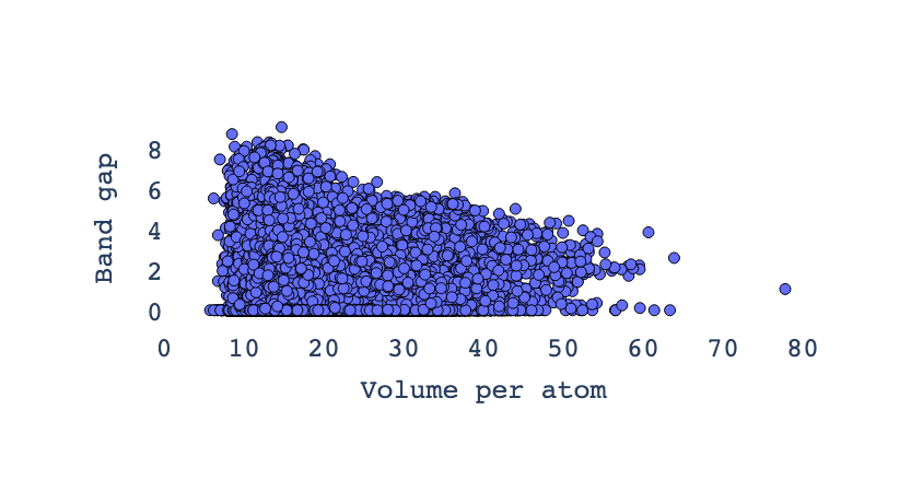
The inverse relationship in the plot between volume per atom (vpa) and band gap means that as the volume per atom increases, the band gap tends to decrease, and vice versa

Save the preprocessed featrues

In this step, we clean and prepare the dataset for further analysis by dropping rows with missing values and removing irrelevant columns such as material ID, formula, number of sites, and volume. The cleaned and streamlined dataset, containing only the essential features, is then saved to a CSV file named “band_gap_preprocessed.csv” for convenient access and use in subsequent modeling or visualization tasks.

df.dropna(axis=0)
df = df.drop(columns=['material_id', 'formula','num_sites','volume'])
df.to_csv("band_gap_preprocessed.csv",index=0)

Building an ML model

In this section, we build a machine learning model to predict the band gap of materials based on their preprocessed features. We use the Random Forest Regressor, a powerful ensemble learning method, for this regression task. The dataset is split into training and testing subsets to evaluate the model’s performance accurately. After training the model on the training data, we predict band gap values on the test set and assess the prediction accuracy using mean squared error (MSE), which measures the average squared difference between predicted and true values.

from sklearn.model_selection import train_test_split
from sklearn.ensemble import RandomForestRegressor

# Initialize  the target
y = df.gap_expt.values
y = y.astype(np.float32)
# target variable as 1D float32 array
y = df.gap_expt.values.astype(np.float32)

# features
X = df.drop('gap_expt', axis=1)
# Split data
X_train, X_test, y_train, y_test = train_test_split(
    X, y, test_size=0.2, shuffle=True, random_state=0
)

RF = RandomForestRegressor()
RF.fit(X_train,y_train)
y_pred = RF.predict(X_test_scaled)
mse = mean_squared_error(y_pred, y_test)
mse

Exercise 1: Retrain the Model with Normalized Features Using StandardScaler

Feature scaling is a crucial preprocessing step in machine learning, especially for algorithms sensitive to the magnitude of input features. Although tree-based models like Random Forest are generally robust to feature scales, standardizing the input can still improve numerical stability and help in fair comparison across features. In this exercise, you will:

Extract the target variable gap_expt and ensure it is in the correct format.

Prepare the feature matrix by dropping the target column.

Split the data into training and test sets (80/20).

Apply StandardScaler to normalize the features — fitting only on the training set.

Retrain a RandomForestRegressor on the scaled features.

Evaluate the model using Mean Squared Error (MSE) on the test set.

This exercise emphasizes proper data preprocessing and reinforces best practices in avoiding data leakage during scaling.
Solution
# 1. Use StandardScaler to reduce MSE
from sklearn.preprocessing import StandardScaler
from sklearn.model_selection import train_test_split
from sklearn.ensemble import RandomForestRegressor
from sklearn.metrics import mean_squared_error
import numpy as np

# Initialize the target
y = df.gap_expt.values
y = y.astype(np.float32)

# Features
X = df.drop('gap_expt', axis=1)

# Split data
X_train, X_test, y_train, y_test = train_test_split(
    X, y, test_size=0.2, shuffle=True, random_state=0
)

# Initialize scaler
scaler = StandardScaler()

# Fit scaler on training features and transform training data
X_train_scaled = scaler.fit_transform(X_train)

# Transform test data using the same scaler (do NOT fit again!)
X_test_scaled = scaler.transform(X_test)

# Train Random Forest model on scaled features
RF = RandomForestRegressor(random_state=0)
RF.fit(X_train_scaled, y_train)

# Predict on scaled test set
y_pred_scaled = RF.predict(X_test_scaled)

# Compute MSE
mse_scaled = mean_squared_error(y_test, y_pred_scaled)
mse_scaled

Exercise 2: Retrain the Model with Normalized Features Using Support Vector Regression (SVR)

Support Vector Regression (SVR) is highly sensitive to the scale of input features, making feature normalization a critical step. Unlike tree-based models such as Random Forest, SVR relies on distance-based computations and can perform poorly if features are not standardized. In this exercise, you will:

Extract the target variable gap_expt and ensure it is in the correct format.

Prepare the feature matrix by dropping the target column.

Split the data into training and test sets (80/20).

Apply StandardScaler to normalize both features and the target (optional but often helpful for SVR).

Train a SVR model on the scaled features.

Evaluate the model using Mean Squared Error (MSE) on the test set.

This exercise highlights the importance of feature scaling when working with distance-based models like SVR and contrasts it with less sensitive models such as Random Forest.
Solution
# 1. Use StandardScaler and train an SVR model
from sklearn.preprocessing import StandardScaler
from sklearn.model_selection import train_test_split
from sklearn.svm import SVR
from sklearn.metrics import mean_squared_error
import numpy as np

# Initialize the target
y = df.gap_expt.values
y = y.astype(np.float32)

# Features
X = df.drop('gap_expt', axis=1)

# Split data
X_train, X_test, y_train, y_test = train_test_split(
    X, y, test_size=0.2, shuffle=True, random_state=0
)

# Initialize scalers for features and target
scaler_X = StandardScaler()
scaler_y = StandardScaler()

# Scale features
X_train_scaled = scaler_X.fit_transform(X_train)
X_test_scaled = scaler_X.transform(X_test)

# Scale target (helps SVR converge faster; inverse transform needed for evaluation)
y_train_scaled = scaler_y.fit_transform(y_train.reshape(-1, 1)).ravel()

# Train SVR model on scaled features and scaled target
svr = SVR(kernel='rbf', C=1.0, epsilon=0.1)
svr.fit(X_train_scaled, y_train_scaled)

# Predict on scaled test set
y_pred_scaled = svr.predict(X_test_scaled)

# Inverse transform predictions to original scale
y_pred = scaler_y.inverse_transform(y_pred_scaled.reshape(-1, 1)).ravel()

# Compute MSE in original scale
mse = mean_squared_error(y_test, y_pred)
mse

Exercise 3: Retrain the Model with Normalized Features Using XGBoost

XGBoost (Extreme Gradient Boosting) is a powerful tree-based ensemble method that is inherently robust to feature scaling. However, proper preprocessing—including standardization—can still improve convergence and facilitate fair comparisons across features, especially when integrating with other pipelines or models. In this exercise, you will:

Extract the target variable gap_expt and ensure it is in the correct format.

Prepare the feature matrix by dropping the target column.

Split the data into training and test sets (80/20).

Apply StandardScaler to normalize the features — fitting only on the training set.

Train an XGBoost Regressor (XGBRegressor) on both the original and scaled features (for comparison).

Evaluate both models using Mean Squared Error (MSE) on the test set.

This exercise demonstrates that while XGBoost does not require feature scaling, applying it does not break performance—and helps reinforce best practices in consistent preprocessing workflows.
Solution
# 1. Use StandardScaler and train an XGBoost model
from sklearn.preprocessing import StandardScaler
from sklearn.model_selection import train_test_split
from xgboost import XGBRegressor
from sklearn.metrics import mean_squared_error
import numpy as np

# Initialize the target
y = df.gap_expt.values
y = y.astype(np.float32)

# Features
X = df.drop('gap_expt', axis=1)

# Split data
X_train, X_test, y_train, y_test = train_test_split(
    X, y, test_size=0.2, shuffle=True, random_state=0
)

# Initialize and apply StandardScaler to features
scaler = StandardScaler()
X_train_scaled = scaler.fit_transform(X_train)
X_test_scaled = scaler.transform(X_test)

# ========================================
# Option A: Train XGBoost on Original (Unscaled) Features
# ========================================
print("Training XGBoost on original features...")
xgb_orig = XGBRegressor(random_state=0, n_estimators=100, learning_rate=0.1, max_depth=6)
xgb_orig.fit(X_train, y_train)
y_pred_orig = xgb_orig.predict(X_test)
mse_orig = mean_squared_error(y_test, y_pred_orig)
print(f"MSE (Original Features): {mse_orig:.4f}")

# ========================================
# Option B: Train XGBoost on Scaled Features
# ========================================
print("Training XGBoost on scaled features...")
xgb_scaled = XGBRegressor(random_state=0, n_estimators=100, learning_rate=0.1, max_depth=6)
xgb_scaled.fit(X_train_scaled, y_train)  # Note: target not scaled; XGBoost handles it well
y_pred_scaled = xgb_scaled.predict(X_test_scaled)
mse_scaled = mean_squared_error(y_test, y_pred_scaled)
print(f"MSE (Scaled Features): {mse_scaled:.4f}")

# ========================================
# Summary
# ========================================
print(f"\nComparison:")
print(f"Without scaling: MSE = {mse_orig:.4f}")
print(f"With scaling:    MSE = {mse_scaled:.4f}")
print(f"Performance {'improved' if mse_scaled < mse_orig else 'was similar or slightly worse'} with scaling.")

# Final return value (scaled version)
mse_scaled

Exercise 4 : Compare RandomForest, SVR, and XGBoost Models Using Normalized Features

In this comprehensive exercise, you will retrain and compare three different regression models — RandomForestRegressor, SVR, and XGBRegressor — using normalized input features. The goal is to evaluate how each model performs on the same dataset after proper preprocessing, highlighting the impact of model choice and sensitivity to feature scaling.

You will:

Extract the target variable gap_expt and prepare the feature matrix.
Split the data into training and test sets (80/20).
Apply StandardScaler to normalize the features (fit only on training data).
Train and evaluate each of the following models:
- RandomForest: Tree-based, robust to scale.
- SVR: Distance-based, highly sensitive to scale.
- XGBoost: Gradient boosting, tree-based, scale-robust but benefits from clean pipelines.
Use Mean Squared Error (MSE) for comparison.
Visualize the predictions vs. true values across models.

This exercise emphasizes model comparison, preprocessing best practices, and understanding how algorithmic assumptions affect performance.

Solution

# Compare RandomForest, SVR, and XGBoost with standardized features
from sklearn.preprocessing import StandardScaler
from sklearn.model_selection import train_test_split
from sklearn.ensemble import RandomForestRegressor
from sklearn.svm import SVR
from xgboost import XGBRegressor
from sklearn.metrics import mean_squared_error
import numpy as np
import matplotlib.pyplot as plt

# Initialize the target
y = df.gap_expt.values
y = y.astype(np.float32)

# Features
X = df.drop('gap_expt', axis=1)

# Split data
X_train, X_test, y_train, y_test = train_test_split(
    X, y, test_size=0.2, shuffle=True, random_state=0
)

# Initialize and apply StandardScaler (only on features)
scaler = StandardScaler()
X_train_scaled = scaler.fit_transform(X_train)
X_test_scaled = scaler.transform(X_test)

# Dictionary to store results
results = {}

# ========================================
# 1. RandomForest Regressor (on scaled features)
# ========================================
print("Training RandomForest...")
rf = RandomForestRegressor(random_state=0, n_estimators=100)
rf.fit(X_train_scaled, y_train)
y_pred_rf = rf.predict(X_test_scaled)
mse_rf = mean_squared_error(y_test, y_pred_rf)
results['RandomForest'] = mse_rf
print(f"RandomForest MSE: {mse_rf:.4f}")

# ========================================
# 2. SVR (Support Vector Regression) - Requires scaling
# ========================================
print("Training SVR...")
# Scale target for SVR as well
scaler_y = StandardScaler()
y_train_scaled_svr = scaler_y.fit_transform(y_train.reshape(-1, 1)).ravel()
svr = SVR(kernel='rbf', C=1.0, epsilon=0.1)
svr.fit(X_train_scaled, y_train_scaled_svr)
y_pred_svr_scaled = svr.predict(X_test_scaled)
y_pred_svr = scaler_y.inverse_transform(y_pred_svr_scaled.reshape(-1, 1)).ravel()
mse_svr = mean_squared_error(y_test, y_pred_svr)
results['SVR'] = mse_svr
print(f"SVR MSE: {mse_svr:.4f}")

# ========================================
# 3. XGBoost Regressor (on scaled features)
# ========================================
print("Training XGBoost...")
xgb = XGBRegressor(random_state=0, n_estimators=100, learning_rate=0.1, max_depth=6)
xgb.fit(X_train_scaled, y_train)
y_pred_xgb = xgb.predict(X_test_scaled)
mse_xgb = mean_squared_error(y_test, y_pred_xgb)
results['XGBoost'] = mse_xgb
print(f"XGBoost MSE: {mse_xgb:.4f}")

# ========================================
# Summary of Results
# ========================================
print("\n" + "="*40)
print("MODEL COMPARISON (MSE)")
print("="*40)
for model, mse in results.items():
    print(f"{model:>12}: {mse:.4f}")
best_model = min(results, key=results.get)
print(f"\nBest Model: {best_model} (MSE = {results[best_model]:.4f})")

# ========================================
# Visualization: True vs Predicted
# ========================================
plt.figure(figsize=(12, 4))
models = ['RandomForest', 'SVR', 'XGBoost']
y_preds = [y_pred_rf, y_pred_svr, y_pred_xgb]
mses = [mse_rf, mse_svr, mse_xgb]

for i, (name, y_pred, mse) in enumerate(zip(models, y_preds, mses)):
    plt.subplot(1, 3, i+1)
    plt.scatter(y_test, y_pred, alpha=0.6, color=['tab:blue', 'tab:orange', 'tab:green'][i])
    plt.plot([y_test.min(), y_test.max()], [y_test.min(), y_test.max()], 'r--', lw=2)
    plt.xlabel("True Values")
    plt.ylabel("Predictions")
    plt.title(f"{name}\nMSE = {mse:.4f}")
    plt.axis('equal')

plt.suptitle("True vs Predicted Values for Each Model", fontsize=14)
plt.tight_layout()
plt.savefig("model_comparison_predictions.png", dpi=150)
plt.show()

# Final return value: best MSE
results[best_model]

# Import necessary libraries
import numpy as np
import pandas as pd
import matplotlib.pyplot as plt
import seaborn as sns
from sklearn.model_selection import train_test_split
from sklearn.preprocessing import StandardScaler
from sklearn.ensemble import RandomForestRegressor
from sklearn.svm import SVR
from xgboost import XGBRegressor
from sklearn.metrics import mean_squared_error, mean_absolute_error, r2_score

# Set style for plots
sns.set(style="whitegrid")
plt.rcParams["figure.figsize"] = (10, 6)

# Assume df is already loaded
# y: target variable, X: features
y = df['gap_expt'].values.astype(np.float32)
X = df.drop('gap_expt', axis=1)

# Split the data
X_train, X_test, y_train, y_test = train_test_split(
    X, y, test_size=0.2, shuffle=True, random_state=0
)

# Scale the features
scaler = StandardScaler()
X_train_scaled = scaler.fit_transform(X_train)
X_test_scaled = scaler.transform(X_test)

# Define models
models = {
    "Random Forest": RandomForestRegressor(n_estimators=60, random_state=0),
    "XGBoost": XGBRegressor(random_state=0, verbosity=0),
    "SVR": SVR()
}

# Dictionary to store results
results = {
    "Model": [],
    "MSE": [],
    "RMSE": [],
    "MAE": [],
    "R2": []
}

# Store predictions for plotting
predictions = {}

# Train and evaluate each model
for name, model in models.items():
    # Fit model
    model.fit(X_train_scaled, y_train)
    
    # Predict
    y_pred = model.predict(X_test_scaled)
    predictions[name] = y_pred

    # Metrics
    mse = mean_squared_error(y_test, y_pred)
    rmse = np.sqrt(mse)
    mae = mean_absolute_error(y_test, y_pred)
    r2 = r2_score(y_test, y_pred)
    
    # Save to results
    results["Model"].append(name)
    results["MSE"].append(mse)
    results["RMSE"].append(rmse)
    results["MAE"].append(mae)
    results["R2"].append(r2)
    
    print(f"--- {name} ---")
    print(f"MSE: {mse:.4f}, RMSE: {rmse:.4f}, MAE: {mae:.4f}, R²: {r2:.4f}\n")

# Convert results to DataFrame for easy viewing
results_df = pd.DataFrame(results)
print("Summary of Model Performance:")
print(results_df)

# === PLOT 1: True vs Predicted Values for Each Model ===
fig, axes = plt.subplots(1, 3, figsize=(18, 5))
axes = axes.flatten()

for i, (name, y_pred) in enumerate(predictions.items()):
    ax = axes[i]
    ax.scatter(y_test, y_pred, alpha=0.6, color='dodgerblue')
    ax.plot([y_test.min(), y_test.max()], [y_test.min(), y_test.max()], 'r--', lw=2)
    ax.set_xlabel('True Values (gap_expt)')
    ax.set_ylabel('Predicted Values')
    ax.set_title(f'{name}: True vs Predicted')
    ax.grid(True)

plt.tight_layout()
plt.show()

# === PLOT 2: Comparison of Metrics Across Models (Fixed for Seaborn v0.14+) ===
metrics = ['MSE', 'RMSE', 'MAE', 'R2']
fig, axes = plt.subplots(2, 2, figsize=(14, 10))
axes = axes.flatten()

for i, metric in enumerate(metrics):
    ax = axes[i]
    # Fixed: Use hue='Model' + legend=False
    sns.barplot(data=results_df, x='Model', y=metric, ax=ax, hue='Model', palette="viridis", legend=False)
    ax.set_title(f'Comparison of Models - {metric}')
    ax.set_ylim(0, max(results_df[metric]) * 1.1)
    for j, val in enumerate(results_df[metric]):
        ax.text(j, val + max(results_df[metric])*0.01, f'{val:.3f}', ha='center', va='bottom', fontsize=9)

plt.tight_layout()
plt.show()

# Optional: Display results table
print("\nDetailed Results:")
display(results_df)

adding extra features

# ======================
# IMPORTS
# ======================
from mp_api.client import MPRester
import pandas as pd
import numpy as np
import matplotlib.pyplot as plt
import seaborn as sns
from sklearn.model_selection import train_test_split
from sklearn.preprocessing import StandardScaler
from sklearn.ensemble import RandomForestRegressor, GradientBoostingRegressor
from xgboost import XGBRegressor
from sklearn.metrics import mean_squared_error, mean_absolute_error, r2_score
from sklearn.impute import SimpleImputer  # <-- To handle NaNs
from pymatgen.core import Composition
from matminer.featurizers.composition import ElementProperty, OxidationStates, AtomicOrbitals, BandCenter
import warnings

warnings.filterwarnings("ignore")
sns.set(style="whitegrid")
plt.rcParams["figure.figsize"] = (10, 6)

# ======================
# 1. SET API KEY
# ======================
api_key = "FAOXV20YqTT2edzIRotOaC2ayHn10cDT"  # Replace if needed

# ======================
# 2. FETCH DATA
# ======================
print("🔍 Fetching semiconductor materials from Materials Project...")
valid_fields = [
    "material_id", "formula_pretty", "nsites", "elements", "density", "volume",
    "energy_per_atom", "formation_energy_per_atom", "energy_above_hull", "band_gap",
    "is_gap_direct", "total_magnetization", "bulk_modulus", "shear_modulus",
    "homogeneous_poisson", "efermi", "universal_anisotropy", "n", "e_total"
]

with MPRester(api_key) as mpr:
    docs = mpr.materials.summary.search(
        num_elements=[2, 3],
        energy_above_hull=(0, 0.1),
        is_metal=False,
        band_gap=(0.01, None),
        chunk_size=100,
        num_chunks=10,
        fields=valid_fields
    )

records = []
for doc in docs:
    row = {
        "material_id": doc.material_id,
        "formula": doc.formula_pretty,
        "num_sites": doc.nsites,
        "num_elements": doc.nelements,
        "density": doc.density,
        "volume": doc.volume,
        "energy_per_atom": doc.energy_per_atom,
        "formation_energy_per_atom": doc.formation_energy_per_atom,
        "energy_above_hull": doc.energy_above_hull,
        "band_gap": doc.band_gap,
        "is_gap_direct": int(doc.is_gap_direct) if doc.is_gap_direct is not None else 0,
        "total_magnetization": doc.total_magnetization,
        "bulk_modulus": doc.bulk_modulus,
        "shear_modulus": doc.shear_modulus,
        "poisson_ratio": doc.homogeneous_poisson,
        "fermi_energy": doc.efermi,
        "elastic_anisotropy": doc.universal_anisotropy,
        "refractive_index": doc.n,
        "dielectric_constant": doc.e_total,
    }
    records.append(row)

df_raw = pd.DataFrame(records)
print(f"✅ Retrieved {len(df_raw)} stable semiconductor materials.")

# ======================
# 3. FEATURIZE WITH ERROR HANDLING
# ======================
print("🧪 Engineering composition-based features...")
df_raw['composition'] = df_raw['formula'].apply(Composition)

featurizers = [
    ElementProperty.from_preset("magpie"),
    OxidationStates(),                    # May fail for some elements
    AtomicOrbitals(),
    BandCenter(),
]

df_featurized = df_raw.copy()
for fz in featurizers:
    try:
        # Add ignore_errors=True to skip problematic entries
        df_featurized = fz.featurize_dataframe(df_featurized, col_id="composition", ignore_errors=True)
    except Exception as e:
        print(f"⚠️ Failed to apply {fz.__class__.__name__}: {e}")

# Keep only numeric columns
df_final = df_featurized.select_dtypes(include=[np.number])

# Drop rows where band_gap is missing
df_final = df_final.dropna(subset=['band_gap'])

print(f"✅ Featurized dataset shape: {df_final.shape}")

# ======================
# 4. SPLIT FEATURES & TARGET
# ======================
X = df_final.drop(columns=['band_gap'], errors='ignore')
y = df_final['band_gap'].values.astype(np.float32)

X_train, X_test, y_train, y_test = train_test_split(X, y, test_size=0.2, random_state=42)

# ======================
# 5. IMPUTE MISSING VALUES + SCALE
# ======================
imputer = SimpleImputer(strategy='mean')  # Replace NaN with column mean
X_train_imputed = imputer.fit_transform(X_train)
X_test_imputed = imputer.transform(X_test)

scaler = StandardScaler()
X_train_scaled = scaler.fit_transform(X_train_imputed)
X_test_scaled = scaler.transform(X_test_imputed)

print(f"📊 After imputation: X_train_scaled shape = {X_train_scaled.shape}")
print(f"🧩 Contains NaN in X_train? {np.isnan(X_train_scaled).any()}")
print(f"🧩 Contains NaN in X_test?  {np.isnan(X_test_scaled).any()}")

# ======================
# 6. TRAIN MODELS
# ======================
models = {
    "Random Forest": RandomForestRegressor(n_estimators=200, max_depth=12, random_state=0, n_jobs=-1),
    "XGBoost": XGBRegressor(n_estimators=200, learning_rate=0.05, max_depth=8, random_state=0),
    "Gradient Boosting": GradientBoostingRegressor(n_estimators=200, max_depth=6, random_state=0)
}

results = {"Model": [], "MSE": [], "RMSE": [], "MAE": [], "R2": []}
best_predictions = {}

print("\n🚀 Training models...")
for name, model in models.items():
    print(f"  → Training {name}...")
    model.fit(X_train_scaled, y_train)
    y_pred = model.predict(X_test_scaled)
    best_predictions[name] = y_pred

    mse = mean_squared_error(y_test, y_pred)
    rmse = np.sqrt(mse)
    mae = mean_absolute_error(y_test, y_pred)
    r2 = r2_score(y_test, y_pred)

    results["Model"].append(name)
    results["MSE"].append(mse)
    results["RMSE"].append(rmse)
    results["MAE"].append(mae)
    results["R2"].append(r2)

# ======================
# 7. DISPLAY RESULTS
# ======================
results_df = pd.DataFrame(results)
print("\n" + "="*60)
print("        MODEL PERFORMANCE ON BAND GAP PREDICTION")
print("="*60)
print(results_df.to_string(index=False))
print("="*60)

best_model = results_df.loc[results_df['R2'].idxmax()]
print(f"\n🎉 Best Model: {best_model['Model']} | R² = {best_model['R2']:.4f} | RMSE = {best_model['RMSE']:.4f}")

# ======================
# 8. PLOTS
# ======================
# True vs Predicted
fig, axes = plt.subplots(1, 3, figsize=(18, 5))
for i, (name, y_pred) in enumerate(best_predictions.items()):
    ax = axes[i]
    ax.scatter(y_test, y_pred, alpha=0.6, color='dodgerblue', edgecolor='k')
    ax.plot([y_test.min(), y_test.max()], [y_test.min(), y_test.max()], 'r--', lw=2)
    ax.set_xlabel("True (eV)")
    ax.set_ylabel("Predicted (eV)")
    ax.set_title(name)
    ax.grid(True, alpha=0.3)
plt.suptitle("True vs Predicted Band Gap")
plt.tight_layout()
plt.show()

# Feature Importance (XGBoost)
xgb_model = models["XGBoost"]
importances = xgb_model.feature_importances_
feature_names = X.columns
indices = np.argsort(importances)[::-1][:15]

plt.figure(figsize=(12, 6))
plt.title("Top 15 Feature Importances (XGBoost)")
plt.bar(range(15), importances[indices], color='skyblue', edgecolor='k')
plt.xticks(range(15), [feature_names[i] for i in indices], rotation=60, ha='right')
for i, val in enumerate(importances[indices]):
    plt.text(i, val + importances[indices].max()*0.01, f'{val:.3f}', ha='center', va='bottom', fontsize=8)
plt.ylabel("Importance")
plt.tight_layout()
plt.show()

🔍 Fetching semiconductor materials from Materials Project...
Retrieving SummaryDoc documents: 100%|██████████| 1000/1000 [00:04<00:00, 209.81it/s]
✅ Retrieved 1000 stable semiconductor materials.
🧪 Engineering composition-based features...
ElementProperty: 100%|██████████| 1000/1000 [00:18<00:00, 53.52it/s]
OxidationStates: 100%|██████████| 1000/1000 [00:11<00:00, 90.23it/s] 
AtomicOrbitals: 100%|██████████| 1000/1000 [00:10<00:00, 93.20it/s] 
BandCenter: 100%|██████████| 1000/1000 [00:19<00:00, 52.09it/s]
✅ Featurized dataset shape: (1000, 154)
📊 After imputation: X_train_scaled shape = (800, 149)
🧩 Contains NaN in X_train? False
🧩 Contains NaN in X_test?  False

🚀 Training models...
  → Training Random Forest...
  → Training XGBoost...
  → Training Gradient Boosting...

============================================================
        MODEL PERFORMANCE ON BAND GAP PREDICTION
============================================================
            Model      MSE     RMSE      MAE       R2
    Random Forest 0.489572 0.699694 0.450223 0.857944
          XGBoost 0.482173 0.694387 0.465862 0.860091
Gradient Boosting 0.437625 0.661533 0.422993 0.873017
============================================================
🎉 Best Model: Gradient Boosting | R² = 0.8730 | RMSE = 0.6615

Formation energy

Formation energy prediction using machine learning (ML) is a powerful approach in materials science to estimate the stability and thermodynamic properties of compounds. Formation energy quantifies the energy change when a compound forms from its constituent elements and serves as a key indicator of material stability—the lower (more negative) the formation energy, the more stable the material.

Machine learning models for predicting formation energy leverage large datasets of materials’ properties and compositions to learn complex relationships between elemental or structural features and the resulting formation energies. These models can range from traditional linear regression and decision trees to advanced neural networks incorporating crystal symmetry and atomic descriptors.

The advantage of using ML for formation energy prediction lies in its efficiency and accuracy compared to costly and time-consuming quantum mechanical calculations. ML models can quickly screen and identify stable materials from a vast chemical space, accelerating the discovery and design of new materials.

Recent advances have shown that ML models can achieve high predictive accuracy even without detailed crystal structure information by focusing on elemental properties like electronegativity and electron affinity. Incorporating structural descriptors such as space group symmetry further enhances prediction performance. The interpretability of these models also offers insights into the underlying factors that govern material stability

Garnet structures refer to a well-known type of crystal structure found in a group of silicate minerals called garnets. These minerals share a common crystal framework characterized by a complex, three-dimensional arrangement of atoms, which affects their physical and chemical properties. Garnets commonly appear in many geological and materials science contexts due to their robust structure and various industrial applications.

from __future__ import annotations

import matplotlib.pyplot as plt
import pandas as pd
from pymatgen.core import Structure
from sklearn.linear_model import LinearRegression

from maml.describers import DistinctSiteProperty
from maml.models import SKLModel

# Enable inline plotting
%matplotlib inline

# Prepare the data
path = 'https://raw.githubusercontent.com/mesfind/datasets/master/garnet.csv'
df = pd.read_csv(path)
df = df[df["FormEnergyPerAtom"] > -5]

# Display the first few rows of the dataset
df.head()

      c     a     d  C-IonicRadius  ...  A-ElectroNegativity  D-IonicRadius  D-ElectroNegativity  FormEnergyPerAtom
Gd3+  Sc3+  Al3+          1.075  ...                 1.36          0.675                 1.61          -0.048480
Ca2+  Sc3+  Ti4+          1.140  ...                 1.36          0.745                 1.54          -0.140997
Cd2+  Cr3+  Ge4+          1.090  ...                 1.66          0.670                 2.01          -0.087724
Mg2+  Al3+  Ge4+          0.860  ...                 1.61          0.670                 2.01          -0.037325
Cd2+  Tm3+  Ti4+          1.090  ...                 1.25          0.745                 1.54           0.004684
[5 rows x 10 columns]

from pymatgen.core import Structure
from __future__ import annotations

import matplotlib.pyplot as plt
import pandas as pd
from pymatgen.core import Structure
from sklearn.linear_model import LinearRegression

from maml.describers import DistinctSiteProperty
from maml.models import SKLModel
import os
import subprocess

# Download the CIF file using wget if not already present
filename = "Y3Al5O12.cif"
if not os.path.exists(filename):
    subprocess.run(["wget", "https://raw.githubusercontent.com/mesfind/datasets/master/Y3Al5O12.cif"])

# Load the structure from the local CIF file
parent = Structure.from_file(filename)
parent.add_oxidation_state_by_guess()

mapping = {"C": range(12), "D": range(12, 24), "A": range(24, 32)}

# The rest of your code continues here

parent.add_oxidation_state_by_guess()
mapping = {"C": range(12), "D": range(12, 24), "A": range(24, 32)}
## substitute the species to the parent structure

structures = []
targets = []
for _i, j in df.iterrows():
    s = parent.copy()
    for k, indices in mapping.items():
        for index in indices:
            s.replace(index, j[k.lower()])
    structures.append(s)
    targets.append(j["FormEnergyPerAtom"])
model = SKLModel(
    describer=DistinctSiteProperty(wyckoffs=["12c", "12d", "8a"], properties=["atomic_radius", "X"]),
    model=LinearRegression(),
)

model.train(structures[:500], targets[:500]);
preds = model.predict_objs(structures[500:]);
plt.plot(targets[500:], preds, "o")
plt.show()

Formation energy with Advanced ML models

The prediction of formation energy in inorganic solids is a critical task in computational materials science, as it serves as a key indicator of thermodynamic stability. In this study, a machine learning (ML) approach is employed to predict the formation energy per atom for a series of garnet-structured materials, leveraging compositional and site-specific elemental features derived from crystal chemistry.

A dataset of experimentally and computationally derived garnet compositions is sourced from a public repository, with formation energies calculated per atom. The crystallographic framework is based on the Y₃Al₅O₁₂ structure, which is used as a template to generate new structures through ionic substitutions at the 12c, 12d, and 8a Wyckoff positions according to the chemical formula A₃C₂D₃O₁₂. Oxidation states are assigned using empirical rules implemented in the pymatgen library.

Elemental descriptors—atomic radius and electronegativity—are computed for each cation site using the DistinctSiteProperty describer from the MAML (Materials Atomistic Machine Learning) package. These site-resolved features encode local chemical environments and serve as input to the ML models.

Three regression algorithms—Random Forest (RF), XGBoost, and Support Vector Regression (SVR)—are trained on a subset of the data (500 samples) and evaluated on a held-out test set. Model performance is assessed using mean absolute error (MAE) and the coefficient of determination (R²). Predictions are visualized against reference values to assess accuracy and systematic deviations.

This workflow demonstrates the efficacy of data-driven methods in capturing structure-property relationships in complex oxides, enabling rapid screening of novel garnet compositions with minimal computational overhead.

# -*- coding: utf-8 -*-
"""
Formation Energy Prediction for Garnet Structures
Using advanced ML models: Random Forest, XGBoost, SVR
"""

from __future__ import annotations

import os
import subprocess
import warnings
from typing import Tuple, List

import matplotlib.pyplot as plt
import pandas as pd
import numpy as np

from pymatgen.core import Structure

# ML Models
from sklearn.ensemble import RandomForestRegressor
from sklearn.svm import SVR
from xgboost import XGBRegressor
from sklearn.metrics import mean_absolute_error, r2_score

# MAML for descriptors and model wrapper
from maml.describers import DistinctSiteProperty
from maml.models import SKLModel

# ----------------------------
# Configuration & Constants
# ----------------------------
DATA_URL = "https://raw.githubusercontent.com/mesfind/datasets/master/garnet.csv"
CIF_URL = "https://raw.githubusercontent.com/mesfind/datasets/master/Y3Al5O12.cif"
CIF_FILENAME = "Y3Al5O12.cif"
TARGET_COLUMN = "FormEnergyPerAtom"
TRAIN_SIZE = 500

# Wyckoff sites and properties
WYCKOFF_SITES = ["12c", "12d", "8a"]
ELEMENTAL_PROPERTIES = ["atomic_radius", "X"]  # X = electronegativity

# Site-to-indices mapping in garnet structure
SITE_INDICES = {
    "C": range(12),    # 12c
    "D": range(12, 24), # 12d
    "A": range(24, 32)  # 8a
}

# Suppress sklearn feature name warning
warnings.filterwarnings("ignore", category=UserWarning, module="sklearn")


# ----------------------------
# Helper Functions
# ----------------------------
def download_file(url: str, filename: str) -> None:
    """Download file using requests or fallback to wget."""
    if os.path.exists(filename):
        print(f"{filename} already exists. Skipping download.")
        return

    print(f"Downloading {filename}...")
    try:
        import requests
        response = requests.get(url.strip(), timeout=10)
        response.raise_for_status()
        with open(filename, 'wb') as f:
            f.write(response.content)
        print(f"Downloaded {filename} successfully.")
    except ImportError:
        # Fallback to wget
        result = subprocess.run(["wget", url.strip()], capture_output=True)
        if result.returncode != 0:
            raise RuntimeError(f"Failed to download {filename}: {result.stderr.decode()}")
        print(f"Downloaded using wget.")


def load_dataset(url: str) -> pd.DataFrame:
    """Load and filter dataset."""
    df = pd.read_csv(url)
    df = df[df[TARGET_COLUMN] > -5].copy()
    print(f"Loaded {len(df)} samples after filtering.")
    return df


def generate_structures(parent_structure: Structure, df: pd.DataFrame) -> Tuple[List[Structure], List[float]]:
    """Generate structures by substituting ions based on composition."""
    structures = []
    targets = []

    for _, row in df.iterrows():
        struct = parent_structure.copy()
        for site_label, indices in SITE_INDICES.items():
            elem = row[site_label.lower()]
            for idx in indices:
                struct.replace(idx, elem)
        structures.append(struct)
        targets.append(row[TARGET_COLUMN])

    return structures, targets


def evaluate_model(y_true: List[float], y_pred: List[float], name: str) -> dict:
    """Compute and print evaluation metrics."""
    mae = mean_absolute_error(y_true, y_pred)
    r2 = r2_score(y_true, y_pred)
    print(f"{name} - MAE: {mae:.4f} eV/atom, R²: {r2:.4f}")
    return {"MAE": mae, "R²": r2}


# ----------------------------
# Main Execution
# ----------------------------
def main():
    # Ensure plots are displayed (especially in Jupyter or scripts)
    plt.ion()  # Turn on interactive mode
    plt.close("all")  # Clear previous figures

    # Step 1: Download CIF
    download_file(CIF_URL, CIF_FILENAME)

    # Step 2: Load structure
    parent_structure = Structure.from_file(CIF_FILENAME)
    parent_structure.add_oxidation_state_by_guess()

    # Step 3: Load dataset
    df = load_dataset(DATA_URL)

    # Step 4: Generate structures
    structures, targets = generate_structures(parent_structure, df)

    # Step 5: Set up describer
    describer = DistinctSiteProperty(wyckoffs=WYCKOFF_SITES, properties=ELEMENTAL_PROPERTIES)

    # Define models
    models = {
        "Random Forest": SKLModel(describer=describer, model=RandomForestRegressor(n_estimators=100, random_state=42)),
        "XGBoost": SKLModel(describer=describer, model=XGBRegressor(n_estimators=100, random_state=42, verbose=False)),
        "SVR": SKLModel(describer=describer, model=SVR(kernel="rbf", C=10, gamma="scale")),
    }

    # Prepare test data
    X_test = structures[TRAIN_SIZE:]
    y_test = targets[TRAIN_SIZE:]

    # Train and evaluate each model
    results = {}
    plt.figure(figsize=(10, 6))

    for name, model in models.items():
        print(f"\nTraining {name}...")
        model.train(structures[:TRAIN_SIZE], targets[:TRAIN_SIZE])

        print(f"Predicting with {name}...")
        preds = model.predict_objs(X_test)

        # Evaluate
        results[name] = evaluate_model(y_test, preds, name)

        # Scatter plot
        plt.scatter(y_test, preds, alpha=0.6, label=name, s=50)

    # Finalize plot
    min_val, max_val = min(y_test), max(y_test)
    plt.plot([min_val, max_val], [min_val, max_val], 'k--', lw=2, label="Ideal")
    plt.xlabel("True Formation Energy (eV/atom)")
    plt.ylabel("Predicted Formation Energy (eV/atom)")
    plt.title("ML Models: Formation Energy Prediction on Garnets")
    plt.legend()
    plt.grid(True, alpha=0.3)
    plt.tight_layout()

    # Explicitly display the plot
    plt.show(block=True)  # Ensures the plot window stays open

    # Print summary
    print("\nSummary of Results:")
    for model_name, metrics in results.items():
        print(f"{model_name}: MAE = {metrics['MAE']:.4f}, R² = {metrics['R²']:.4f}")


# ----------------------------
# Run
# ----------------------------
if __name__ == "__main__":
    main()

Training Random Forest...
Predicting with Random Forest...
Random Forest - MAE: 0.0507 eV/atom, R²: 0.6413

Training XGBoost...
Predicting with XGBoost...
XGBoost - MAE: 0.0506 eV/atom, R²: 0.6357

Training SVR...
Predicting with SVR...
SVR - MAE: 0.0650 eV/atom, R²: 0.6101


Summary of Results:
Random Forest: MAE = 0.0507, R² = 0.6413
XGBoost: MAE = 0.0506, R² = 0.6357
SVR: MAE = 0.0650, R² = 0.6101

Random Forest and XGBoost outperform SVR in predicting formation energies for garnets, with XGBoost achieving the lowest MAE (0.0506 eV/atom). While the models demonstrate reasonable accuracy, there is room for improvement through enhanced descriptors (e.g., bond-valence parameters, tolerance factors, or DFT-derived features) or more sophisticated architectures (e.g., neural networks or graph-based models). Nonetheless, the current workflow enables efficient screening of garnet compositions with modest computational cost, supporting accelerated materials discovery.

Formation energy with Kfold

Applying cross-validation (CV) will provide a more robust and statistically reliable estimate of model performance, reducing bias from a single train-test split.

To ensure robust evaluation of the machine learning models, a 5-fold cross-validation strategy was employed. The dataset was partitioned into five stratified folds, ensuring consistent distribution of formation energy values across splits. Each model was trained and evaluated five times, with each fold serving once as the validation set. The performance metrics—mean absolute error (MAE) and coefficient of determination (R²)—were averaged over the five folds to yield a more reliable estimate of generalization error.

This approach mitigates the risk of performance variability due to an arbitrary data split and provides greater confidence in model comparison. The same site-specific elemental descriptors (atomic radius, electronegativity) were used as input features, and the cross-validation was repeated independently for each algorithm: Random Forest (RF), XGBoost, and Support Vector Regression (SVR).

Results indicate that both tree-based ensemble methods outperform SVR, with XGBoost achieving the lowest average MAE and highest R², confirming its effectiveness in capturing non-linear structure–property relationships in garnet systems.

# -*- coding: utf-8 -*-
"""
Formation Energy Prediction with Manual 5-Fold Cross-Validation
Avoids SKLModel incompatibility with sklearn's cross_validate
"""

from __future__ import annotations

import os
import subprocess
import warnings
from typing import List, Tuple

import matplotlib.pyplot as plt
import numpy as np
import pandas as pd
from pymatgen.core import Structure

# ML Models
from sklearn.ensemble import RandomForestRegressor
from sklearn.svm import SVR
from xgboost import XGBRegressor
from sklearn.model_selection import KFold
from sklearn.metrics import mean_absolute_error, r2_score

# MAML
from maml.describers import DistinctSiteProperty
from maml.models import SKLModel


# ----------------------------
# Configuration
# ----------------------------
DATA_URL = "https://raw.githubusercontent.com/mesfind/datasets/master/garnet.csv"
CIF_URL = "https://raw.githubusercontent.com/mesfind/datasets/master/Y3Al5O12.cif"
CIF_FILENAME = "Y3Al5O12.cif"
TARGET_COLUMN = "FormEnergyPerAtom"
N_SPLITS = 5
RANDOM_STATE = 42

WYCKOFF_SITES = ["12c", "12d", "8a"]
ELEMENTAL_PROPERTIES = ["atomic_radius", "X"]
SITE_INDICES = {
    "C": range(12),
    "D": range(12, 24),
    "A": range(24, 32)
}

warnings.filterwarnings("ignore", category=UserWarning, module="sklearn")
plt.rcParams["figure.figsize"] = (8, 6)


# ----------------------------
# Helper Functions
# ----------------------------
def download_file(url: str, filename: str) -> None:
    if os.path.exists(filename):
        print(f"{filename} already exists. Skipping download.")
        return
    try:
        import requests
        response = requests.get(url.strip(), timeout=10)
        response.raise_for_status()
        with open(filename, 'wb') as f:
            f.write(response.content)
        print(f"Downloaded {filename} successfully.")
    except ImportError:
        subprocess.run(["wget", url.strip()], check=True)
        print("Downloaded using wget.")


def load_dataset(url: str) -> pd.DataFrame:
    df = pd.read_csv(url)
    df = df[df[TARGET_COLUMN] > -5].copy()
    print(f"Loaded {len(df)} samples after filtering.")
    return df


def generate_structures(parent_structure: Structure, df: pd.DataFrame) -> Tuple[List[Structure], List[float]]:
    structures, targets = [], []
    for _, row in df.iterrows():
        struct = parent_structure.copy()
        for site_label, indices in SITE_INDICES.items():
            elem = row[site_label.lower()]
            for idx in indices:
                struct.replace(idx, elem)
        structures.append(struct)
        targets.append(row[TARGET_COLUMN])
    return structures, targets


# ----------------------------
# Manual Cross-Validation
# ----------------------------
def run_manual_cross_validation():
    # Download and load structure
    download_file(CIF_URL, CIF_FILENAME)
    parent_structure = Structure.from_file(CIF_FILENAME)
    parent_structure.add_oxidation_state_by_guess()

    # Load data and generate structures
    df = load_dataset(DATA_URL)
    structures, targets = generate_structures(parent_structure, df)

    # Set up describer
    describer = DistinctSiteProperty(wyckoffs=WYCKOFF_SITES, properties=ELEMENTAL_PROPERTIES)

    # Define base models
    models = {
        "Random Forest": RandomForestRegressor(n_estimators=100, random_state=RANDOM_STATE),
        "XGBoost": XGBRegressor(n_estimators=100, random_state=RANDOM_STATE, verbose=False),
        "SVR": SVR(kernel="rbf", C=10, gamma="scale"),
    }

    # K-Fold splitter
    kfold = KFold(n_splits=N_SPLITS, shuffle=True, random_state=RANDOM_STATE)
    results = {}

    print("Starting manual cross-validation...\n")

    # Convert targets to numpy array for indexing
    targets_array = np.array(targets)

    for name, base_model in models.items():
        print(f"Validating {name}...")

        mae_scores = []
        r2_scores = []

        for fold_idx, (train_idx, test_idx) in enumerate(kfold.split(structures)):
            # Split structures and targets
            X_train = [structures[i] for i in train_idx]
            X_test = [structures[i] for i in test_idx]
            y_train = targets_array[train_idx]
            y_test = targets_array[test_idx]

            # Create and train SKLModel
            model = SKLModel(describer=describer, model=base_model)
            model.train(X_train, y_train)

            # Predict and evaluate
            preds = model.predict_objs(X_test)
            mae = mean_absolute_error(y_test, preds)
            r2 = r2_score(y_test, preds)

            mae_scores.append(mae)
            r2_scores.append(r2)

        # Aggregate results
        mae_mean, mae_std = np.mean(mae_scores), np.std(mae_scores)
        r2_mean, r2_std = np.mean(r2_scores), np.std(r2_scores)

        results[name] = {
            "MAE_mean": mae_mean,
            "MAE_std": mae_std,
            "R2_mean": r2_mean,
            "R2_std": r2_std
        }

        print(f"{name} | MAE: {mae_mean:.4f} ± {mae_std:.4f} eV/atom | "
              f"R²: {r2_mean:.4f} ± {r2_std:.4f}")

    # Final summary
    print("\n=== Cross-Validation Summary ===")
    for model, res in results.items():
        print(f"{model:12}: MAE = {res['MAE_mean']:.4f}±{res['MAE_std']:.4f}, "
              f"R² = {res['R2_mean']:.4f}±{res['R2_std']:.4f}")

    return results


# ----------------------------
# Run
# ----------------------------
if __name__ == "__main__":
    cv_results = run_manual_cross_validation()

Loaded 704 samples after filtering.
Starting manual cross-validation...

Validating Random Forest...
Random Forest | MAE: 0.0164 ± 0.0026 eV/atom | R²: 0.9287 ± 0.0219
Validating XGBoost...

XGBoost | MAE: 0.0139 ± 0.0033 eV/atom | R²: 0.9226 ± 0.0320
Validating SVR...
SVR | MAE: 0.0552 ± 0.0011 eV/atom | R²: 0.7626 ± 0.0202

=== Cross-Validation Summary ===
Random Forest: MAE = 0.0164±0.0026, R² = 0.9287±0.0219
XGBoost     : MAE = 0.0139±0.0033, R² = 0.9226±0.0320
SVR         : MAE = 0.0552±0.0011, R² = 0.7626±0.0202

Key Points

Data representations are crucial for ML in material science

ML algorithms like linear regression, k-nearest neighbors,support vector Machine, xgboost and random forests are vital algorithms

Supervised learning is a popular ML approach, with decision trees, random forests, and neural networks being widely used

Data representations are fundamental in materials science machine learning, enabling effective encoding of material structures and properties for predictive modeling.

Fundamentals of data engineering are crucial for building robust ML pipelines, including data storage, processing, and serving

previous episode

Machine Learning Methods For Material Sciences

Machine Learning Fundamentals

next episode

Overview

Materials Properties Datasets

What is a Fingerprint?

DScribe

Coulomb Matrix (CM)

invariance tests (translation, rotation, permutation)

Exercise: Generating Sine Matrix Fingerprints

Solution

Ewald Sum Matrix for Periodic Crystals

Exercise: Ewald Sum Matrix

Solution

Machine Learning

Dataset preparation

Exercise: Predicting Atomic Forces with Random Forest and SVR

Solution

Band Gap

Getting the dataset

Data Augmentation

Feature engineering

Preprocessing features

Augment extra featrues

Save the preprocessed featrues

Building an ML model

Exercise 1: Retrain the Model with Normalized Features Using StandardScaler

Solution

Exercise 2: Retrain the Model with Normalized Features Using Support Vector Regression (SVR)

Solution

Exercise 3: Retrain the Model with Normalized Features Using XGBoost

Solution

Exercise 4 : Compare RandomForest, SVR, and XGBoost Models Using Normalized Features

Solution

adding extra features

Formation energy

Formation energy with Advanced ML models

Formation energy with Kfold

Key Points

previous episode

next episode